Tag: Decision-Making Models

Normal distribution, or the Gaussian distribution, is a fundamental probability distribution that describes how data values are distributed symmetrically around a mean. Its graph forms a bell-shaped curve, with most data points clustering near the mean and fewer occurring as they deviate further. The curve is defined by two parameters: the mean (μ) and the standard deviation (σ), which determine its center and spread. Normal distribution is widely used in statistics, natural sciences, and social sciences for analysis and inference.

The general form of its probability density function is:

The parameter μ is the mean or expectation of the distribution (and also its median and mode), while the parameter σ is its standard deviation. The variance of the distribution is σ^2. A random variable with a Gaussian distribution is said to be normally distributed, and is called a normal deviate.

Normal distributions are important in statistics and are often used in the natural and social sciences to represent real-valued random variables whose distributions are not known. Their importance is partly due to the central limit theorem. It states that, under some conditions, the average of many samples (observations) of a random variable with finite mean and variance is itself a random variable whose distribution converges to a normal distribution as the number of samples increases. Therefore, physical quantities that are expected to be the sum of many independent processes, such as measurement errors, often have distributions that are nearly normal.

A normal distribution is sometimes informally called a bell curve. However, many other distributions are bell-shaped (such as the Cauchy, Student’s t, and logistic distributions).

Importance of Normal Distribution:

1. Foundation of Statistical Inference

The normal distribution is central to statistical inference. Many parametric tests, such as t-tests and ANOVA, are based on the assumption that the data follows a normal distribution. This simplifies hypothesis testing, confidence interval estimation, and other analytical procedures.

2. Real-Life Data Approximation

Many natural phenomena and datasets, such as heights, weights, IQ scores, and measurement errors, tend to follow a normal distribution. This makes it a practical and realistic model for analyzing real-world data, simplifying interpretation and analysis.

3. Basis for Central Limit Theorem (CLT)

The normal distribution is critical in understanding the Central Limit Theorem, which states that the sampling distribution of the sample mean approaches a normal distribution as the sample size increases, regardless of the population’s actual distribution. This enables statisticians to make predictions and draw conclusions from sample data.

4. Application in Quality Control

In industries, normal distribution is widely used in quality control and process optimization. Control charts and Six Sigma methodologies assume normality to monitor processes and identify deviations or defects effectively.

5. Probability Calculations

The normal distribution allows for the easy calculation of probabilities for different scenarios. Its standardized form, the z-score, simplifies these calculations, making it easier to determine how data points relate to the overall distribution.

6. Modeling Financial and Economic Data

In finance and economics, normal distribution is used to model returns, risks, and forecasts. Although real-world data often exhibit deviations, normal distribution serves as a baseline for constructing more complex models.

Central limit theorem

In probability theory, the central limit theorem (CLT) establishes that, in many situations, when independent random variables are added, their properly normalized sum tends toward a normal distribution (informally a bell curve) even if the original variables themselves are not normally distributed. The theorem is a key concept in probability theory because it implies that probabilistic and statistical methods that work for normal distributions can be applicable to many problems involving other types of distributions. This theorem has seen many changes during the formal development of probability theory. Previous versions of the theorem date back to 1810, but in its modern general form, this fundamental result in probability theory was precisely stated as late as 1920, thereby serving as a bridge between classical and modern probability theory.

Characteristics Fitting a Normal Distribution

Poisson distribution is a probability distribution used to model the number of events occurring within a fixed interval of time, space, or other dimensions, given that these events occur independently and at a constant average rate.

Importance

1. Modeling Rare Events: Used to model the probability of rare events, such as accidents, machine failures, or phone call arrivals.
2. Applications in Various Fields: Applicable in business, biology, telecommunications, and reliability engineering.
3. Simplifies Complex Processes: Helps analyze situations with numerous trials and low probability of success per trial.
4. Foundation for Queuing Theory: Forms the basis for queuing models used in service and manufacturing industries.
5. Approximation of Binomial Distribution: When the number of trials is large, and the probability of success is small, Poisson distribution approximates the binomial distribution.

Conditions for Poisson Distribution

1. Independence: Events must occur independently of each other.
2. Constant Rate: The average rate (λ) of occurrence is constant over time or space.
3. Non-Simultaneous Events: Two events cannot occur simultaneously within the defined interval.
4. Fixed Interval: The observation is within a fixed time, space, or other defined intervals.

Constants

1. Mean (λ): Represents the expected number of events in the interval.
2. Variance (λ): Equal to the mean, reflecting the distribution’s spread.
3. Skewness: The distribution is skewed to the right when λ is small and becomes symmetric as λ increases.
4. Probability Mass Function (PMF): P(X = k) = [e^−λ*λ^k] / k!, Where $k$ is the number of occurrences, $e$ is the base of the natural logarithm, and λ is the mean.

Fitting of Poisson Distribution

When a Poisson distribution is to be fitted to an observed data the following procedure is adopted:

The binomial distribution is a probability distribution that summarizes the likelihood that a value will take one of two independent values under a given set of parameters or assumptions. The underlying assumptions of the binomial distribution are that there is only one outcome for each trial, that each trial has the same probability of success, and that each trial is mutually exclusive, or independent of each other.

In probability theory and statistics, the binomial distribution with parameters n and p is the discrete probability distribution of the number of successes in a sequence of n independent experiments, each asking a yes, no question, and each with its own Boolean-valued outcome: success (with probability p) or failure (with probability q = 1 − p). A single success/failure experiment is also called a Bernoulli trial or Bernoulli experiment, and a sequence of outcomes is called a Bernoulli process; for a single trial, i.e., n = 1, the binomial distribution is a Bernoulli distribution. The binomial distribution is the basis for the popular binomial test of statistical significance.

The binomial distribution is frequently used to model the number of successes in a sample of size n drawn with replacement from a population of size N. If the sampling is carried out without replacement, the draws are not independent and so the resulting distribution is a hypergeometric distribution, not a binomial one. However, for N much larger than n, the binomial distribution remains a good approximation, and is widely used

The binomial distribution is a common discrete distribution used in statistics, as opposed to a continuous distribution, such as the normal distribution. This is because the binomial distribution only counts two states, typically represented as 1 (for a success) or 0 (for a failure) given a number of trials in the data. The binomial distribution, therefore, represents the probability for x successes in n trials, given a success probability p for each trial.

Binomial distribution summarizes the number of trials, or observations when each trial has the same probability of attaining one particular value. The binomial distribution determines the probability of observing a specified number of successful outcomes in a specified number of trials.

The binomial distribution is often used in social science statistics as a building block for models for dichotomous outcome variables, like whether a Republican or Democrat will win an upcoming election or whether an individual will die within a specified period of time, etc.

Importance

For example, adults with allergies might report relief with medication or not, children with a bacterial infection might respond to antibiotic therapy or not, adults who suffer a myocardial infarction might survive the heart attack or not, a medical device such as a coronary stent might be successfully implanted or not. These are just a few examples of applications or processes in which the outcome of interest has two possible values (i.e., it is dichotomous). The two outcomes are often labeled “success” and “failure” with success indicating the presence of the outcome of interest. Note, however, that for many medical and public health questions the outcome or event of interest is the occurrence of disease, which is obviously not really a success. Nevertheless, this terminology is typically used when discussing the binomial distribution model. As a result, whenever using the binomial distribution, we must clearly specify which outcome is the “success” and which is the “failure”.

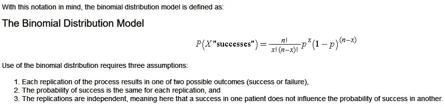
The binomial distribution model allows us to compute the probability of observing a specified number of “successes” when the process is repeated a specific number of times (e.g., in a set of patients) and the outcome for a given patient is either a success or a failure. We must first introduce some notation which is necessary for the binomial distribution model.

First, we let “n” denote the number of observations or the number of times the process is repeated, and “x” denotes the number of “successes” or events of interest occurring during “n” observations. The probability of “success” or occurrence of the outcome of interest is indicated by “p”.

The binomial equation also uses factorials. In mathematics, the factorial of a non-negative integer k is denoted by k!, which is the product of all positive integers less than or equal to k. For example,

• 4! = 4 x 3 x 2 x 1 = 24,
• 2! = 2 x 1 = 2,
• 1!=1.
• There is one special case, 0! = 1.

Conditions

• The number of observations n is fixed.
• Each observation is independent.
• Each observation represents one of two outcomes (“success” or “failure”).
• The probability of “success” p is the same for each outcome

Constants

Fitting of Binomial Distribution

Fitting of probability distribution to a series of observed data helps to predict the probability or to forecast the frequency of occurrence of the required variable in a certain desired interval.

To fit any theoretical distribution, one should know its parameters and probability distribution. Parameters of Binomial distribution are n and p. Once p and n are known, binomial probabilities for different random events and the corresponding expected frequencies can be computed. From the given data we can get n by inspection. For binomial distribution, we know that mean is equal to np hence we can estimate p as = mean/n. Thus, with these n and p one can fit the binomial distribution.

There are many probability distributions of which some can be fitted more closely to the observed frequency of the data than others, depending on the characteristics of the variables. Therefore, one needs to select a distribution that suits the data well.

Sample design is the framework, or road map, that serves as the basis for the selection of a survey sample and affects many other important aspects of a survey as well. In a broad context, survey researchers are interested in obtaining some type of information through a survey for some population, or universe, of interest. One must define a sampling frame that represents the population of interest, from which a sample is to be drawn. The sampling frame may be identical to the population, or it may be only part of it and is therefore subject to some under coverage, or it may have an indirect relationship to the population.

Sampling is the process of selecting a subset of individuals, items, or observations from a larger population to analyze and draw conclusions about the entire group. It is essential in statistics when studying the entire population is impractical, time-consuming, or costly. Sampling can be done using various methods, such as random, stratified, cluster, or systematic sampling. The main objectives of sampling are to ensure representativeness, reduce costs, and provide timely insights. Proper sampling techniques enhance the reliability and validity of statistical analysis and decision-making processes.

Steps in Sample Design

While developing a sampling design, the researcher must pay attention to the following points:

• Type of Universe:

The first step in developing any sample design is to clearly define the set of objects, technically called the Universe, to be studied. The universe can be finite or infinite. In finite universe the number of items is certain, but in case of an infinite universe the number of items is infinite, i.e., we cannot have any idea about the total number of items. The population of a city, the number of workers in a factory and the like are examples of finite universes, whereas the number of stars in the sky, listeners of a specific radio programme, throwing of a dice etc. are examples of infinite universes.

• Sampling unit:

A decision has to be taken concerning a sampling unit before selecting sample. Sampling unit may be a geographical one such as state, district, village, etc., or a construction unit such as house, flat, etc., or it may be a social unit such as family, club, school, etc., or it may be an individual. The researcher will have to decide one or more of such units that he has to select for his study.

• Source list:

It is also known as ‘sampling frame’ from which sample is to be drawn. It contains the names of all items of a universe (in case of finite universe only). If source list is not available, researcher has to prepare it. Such a list should be comprehensive, correct, reliable and appropriate. It is extremely important for the source list to be as representative of the population as possible.

• Size of Sample:

This refers to the number of items to be selected from the universe to constitute a sample. This a major problem before a researcher. The size of sample should neither be excessively large, nor too small. It should be optimum. An optimum sample is one which fulfills the requirements of efficiency, representativeness, reliability and flexibility. While deciding the size of sample, researcher must determine the desired precision as also an acceptable confidence level for the estimate. The size of population variance needs to be considered as in case of larger variance usually a bigger sample is needed. The size of population must be kept in view for this also limits the sample size. The parameters of interest in a research study must be kept in view, while deciding the size of the sample. Costs too dictate the size of sample that we can draw. As such, budgetary constraint must invariably be taken into consideration when we decide the sample size.

• Parameters of interest:

In determining the sample design, one must consider the question of the specific population parameters which are of interest. For instance, we may be interested in estimating the proportion of persons with some characteristic in the population, or we may be interested in knowing some average or the other measure concerning the population. There may also be important sub-groups in the population about whom we would like to make estimates. All this has a strong impact upon the sample design we would accept.

• Budgetary constraint:

Cost considerations, from practical point of view, have a major impact upon decisions relating to not only the size of the sample but also to the type of sample. This fact can even lead to the use of a non-probability sample.

• Sampling procedure:

Finally, the researcher must decide the type of sample he will use i.e., he must decide about the technique to be used in selecting the items for the sample. In fact, this technique or procedure stands for the sample design itself. There are several sample designs (explained in the pages that follow) out of which the researcher must choose one for his study. Obviously, he must select that design which, for a given sample size and for a given cost, has a smaller sampling error.

Types of Samples

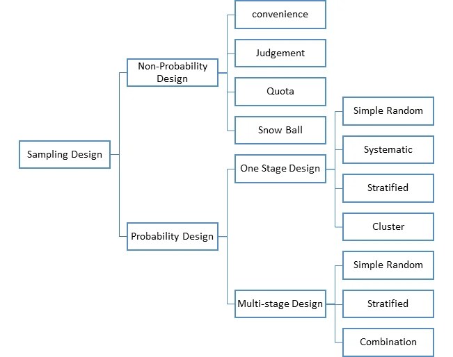
• Probability Sampling (Representative samples)

Probability samples are selected in such a way as to be representative of the population. They provide the most valid or credible results because they reflect the characteristics of the population from which they are selected (e.g., residents of a particular community, students at an elementary school, etc.). There are two types of probability samples: random and stratified.

• Random Sample

The term random has a very precise meaning. Each individual in the population of interest has an equal likelihood of selection. This is a very strict meaning you can’t just collect responses on the street and have a random sample.

The assumption of an equal chance of selection means that sources such as a telephone book or voter registration lists are not adequate for providing a random sample of a community. In both these cases there will be a number of residents whose names are not listed. Telephone surveys get around this problem by random-digit dialling but that assumes that everyone in the population has a telephone. The key to random selection is that there is no bias involved in the selection of the sample. Any variation between the sample characteristics and the population characteristics is only a matter of chance.

• Stratified Sample

A stratified sample is a mini-reproduction of the population. Before sampling, the population is divided into characteristics of importance for the research. For example, by gender, social class, education level, religion, etc. Then the population is randomly sampled within each category or stratum. If 38% of the population is college-educated, then 38% of the sample is randomly selected from the college-educated population.

Stratified samples are as good as or better than random samples, but they require fairly detailed advance knowledge of the population characteristics, and therefore are more difficult to construct.

• Non-probability Samples (Non-representative samples)

As they are not truly representative, non-probability samples are less desirable than probability samples. However, a researcher may not be able to obtain a random or stratified sample, or it may be too expensive. A researcher may not care about generalizing to a larger population. The validity of non-probability samples can be increased by trying to approximate random selection, and by eliminating as many sources of bias as possible.

• Quota Sample

The defining characteristic of a quota sample is that the researcher deliberately sets the proportions of levels or strata within the sample. This is generally done to insure the inclusion of a particular segment of the population. The proportions may or may not differ dramatically from the actual proportion in the population. The researcher sets a quota, independent of population characteristics.

Example: A researcher is interested in the attitudes of members of different religions towards the death penalty. In Iowa a random sample might miss Muslims (because there are not many in that state). To be sure of their inclusion, a researcher could set a quota of 3% Muslim for the sample. However, the sample will no longer be representative of the actual proportions in the population. This may limit generalizing to the state population. But the quota will guarantee that the views of Muslims are represented in the survey.

• Purposive Sample

A purposive sample is a non-representative subset of some larger population, and is constructed to serve a very specific need or purpose. A researcher may have a specific group in mind, such as high level business executives. It may not be possible to specify the population they would not all be known, and access will be difficult. The researcher will attempt to zero in on the target group, interviewing whoever is available.

• Convenience Sample

A convenience sample is a matter of taking what you can get. It is an accidental sample. Although selection may be unguided, it probably is not random, using the correct definition of everyone in the population having an equal chance of being selected. Volunteers would constitute a convenience sample.

Non-probability samples are limited with regard to generalization. Because they do not truly represent a population, we cannot make valid inferences about the larger group from which they are drawn. Validity can be increased by approximating random selection as much as possible, and making every attempt to avoid introducing bias into sample selection.

Sampling Distribution

Sampling Distribution is a statistical concept that describes the probability distribution of a given statistic (e.g., mean, variance, or proportion) derived from repeated random samples of a specific size taken from a population. It plays a crucial role in inferential statistics, providing the foundation for making predictions and drawing conclusions about a population based on sample data.

Concepts of Sampling Distribution

A sampling distribution is the distribution of a statistic (not raw data) over all possible samples of the same size from a population. Commonly used statistics include the sample mean (Xˉ\bar{X}Xˉ), sample variance, and sample proportion.

Purpose:

It allows statisticians to estimate population parameters, test hypotheses, and calculate probabilities for statistical inference.

Shape and Characteristics:

• • The shape of the sampling distribution depends on the population distribution and the sample size.
  • For large sample sizes, the Central Limit Theorem states that the sampling distribution of the mean will be approximately normal, regardless of the population’s distribution.

Importance of Sampling Distribution

• Facilitates Statistical Inference:

Sampling distributions are used to construct confidence intervals and perform hypothesis tests, helping to infer population characteristics.

• Standard Error:

The standard deviation of the sampling distribution, called the standard error, quantifies the variability of the sample statistic. Smaller standard errors indicate more reliable estimates.

• Links Population and Samples:

It provides a theoretical framework that connects sample statistics to population parameters.

Types of Sampling Distributions

• Distribution of Sample Means:

Shows the distribution of means from all possible samples of a population.

• Distribution of Sample Proportions:

Represents the proportion of a certain outcome in samples, used in binomial settings.

• Distribution of Sample Variances:

Explains the variability in sample data.

Example

Consider a population of students’ test scores with a mean of 70 and a standard deviation of 10. If we repeatedly draw random samples of size 30 and calculate the sample mean, the distribution of those means forms the sampling distribution. This distribution will have a mean close to 70 and a reduced standard deviation (standard error).

The range is a measure of dispersion that represents the difference between the highest and lowest values in a dataset. It provides a simple way to understand the spread of data. While easy to calculate, the range is sensitive to outliers and does not provide information about the distribution of values between the extremes.

Range of a distribution gives a measure of the width (or the spread) of the data values of the corresponding random variable. For example, if there are two random variables X and Y such that X corresponds to the age of human beings and Y corresponds to the age of turtles, we know from our general knowledge that the variable corresponding to the age of turtles should be larger.

Since the average age of humans is 50-60 years, while that of turtles is about 150-200 years; the values taken by the random variable Y are indeed spread out from 0 to at least 250 and above; while those of X will have a smaller range. Thus, qualitatively you’ve already understood what the Range of a distribution means. The mathematical formula for the same is given as:

Range = L – S

where

L: The Largets/maximum value attained by the random variable under consideration

S: The smallest/minimum value.

Properties

• The Range of a given distribution has the same units as the data points.
• If a random variable is transformed into a new random variable by a change of scale and a shift of origin as:

Y = aX + b

where

Y: the new random variable

X: the original random variable

a,b: constants.

Then the ranges of X and Y can be related as:

R_Y = |a|R_X

Clearly, the shift in origin doesn’t affect the shape of the distribution, and therefore its spread (or the width) remains unchanged. Only the scaling factor is important.

• For a grouped class distribution, the Range is defined as the difference between the two extreme class boundaries.
• A better measure of the spread of a distribution is the Coefficient of Range, given by:

Coefficient of Range (expressed as a percentage) = L – SL + S × 100

Clearly, we need to take the ratio between the Range and the total (combined) extent of the distribution. Besides, since it is a ratio, it is dimensionless, and can, therefore, one can use it to compare the spreads of two or more different distributions as well.

• The range is an absolute measure of Dispersion of a distribution while the Coefficient of Range is a relative measure of dispersion.

Due to the consideration of only the end-points of a distribution, the Range never gives us any information about the shape of the distribution curve between the extreme points. Thus, we must move on to better measures of dispersion. One such quantity is Mean Deviation which is we are going to discuss now.

Interquartile range (IQR)

The interquartile range is the middle half of the data. To visualize it, think about the median value that splits the dataset in half. Similarly, you can divide the data into quarters. Statisticians refer to these quarters as quartiles and denote them from low to high as Q1, Q2, Q3, and Q4. The lowest quartile (Q1) contains the quarter of the dataset with the smallest values. The upper quartile (Q4) contains the quarter of the dataset with the highest values. The interquartile range is the middle half of the data that is in between the upper and lower quartiles. In other words, the interquartile range includes the 50% of data points that fall in Q2 and

The IQR is the red area in the graph below.

The interquartile range is a robust measure of variability in a similar manner that the median is a robust measure of central tendency. Neither measure is influenced dramatically by outliers because they don’t depend on every value. Additionally, the interquartile range is excellent for skewed distributions, just like the median. As you’ll learn, when you have a normal distribution, the standard deviation tells you the percentage of observations that fall specific distances from the mean. However, this doesn’t work for skewed distributions, and the IQR is a great alternative.

I’ve divided the dataset below into quartiles. The interquartile range (IQR) extends from the low end of Q2 to the upper limit of Q3. For this dataset, the range is 21 – 39.