Baye’s Theorem

Bayes’ Theorem is a way to figure out conditional probability. Conditional probability is the probability of an event happening, given that it has some relationship to one or more other events. For example, your probability of getting a parking space is connected to the time of day you park, where you park, and what conventions are going on at any time. Bayes’ theorem is slightly more nuanced. In a nutshell, it gives you the actual probability of an event given information about tests.

“Events” Are different from “tests.” For example, there is a test for liver disease, but that’s separate from the event of actually having liver disease.

Tests are flawed:

Just because you have a positive test does not mean you actually have the disease. Many tests have a high false positive rate. Rare events tend to have higher false positive rates than more common events. We’re not just talking about medical tests here. For example, spam filtering can have high false positive rates. Bayes’ theorem takes the test results and calculates your real probability that the test has identified the event.

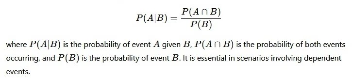
Bayes’ Theorem (also known as Bayes’ rule) is a deceptively simple formula used to calculate conditional probability. The Theorem was named after English mathematician Thomas Bayes (1701-1761). The formal definition for the rule is:

In most cases, you can’t just plug numbers into an equation; You have to figure out what your “tests” and “events” are first. For two events, A and B, Bayes’ theorem allows you to figure out p(A|B) (the probability that event A happened, given that test B was positive) from p(B|A) (the probability that test B happened, given that event A happened). It can be a little tricky to wrap your head around as technically you’re working backwards; you may have to switch your tests and events around, which can get confusing. An example should clarify what I mean by “switch the tests and events around.”

Bayes’ Theorem Example

You might be interested in finding out a patient’s probability of having liver disease if they are an alcoholic. “Being an alcoholic” is the test (kind of like a litmus test) for liver disease.

A could mean the event “Patient has liver disease.” Past data tells you that 10% of patients entering your clinic have liver disease. P(A) = 0.10.

B could mean the litmus test that “Patient is an alcoholic.” Five percent of the clinic’s patients are alcoholics. P(B) = 0.05.

You might also know that among those patients diagnosed with liver disease, 7% are alcoholics. This is your B|A: the probability that a patient is alcoholic, given that they have liver disease, is 7%.

Bayes’ theorem tells you:

P(A|B) = (0.07 * 0.1)/0.05 = 0.14

In other words, if the patient is an alcoholic, their chances of having liver disease is 0.14 (14%). This is a large increase from the 10% suggested by past data. But it’s still unlikely that any particular patient has liver disease.

Indifference Curve Analysis

Indifference curve analysis is basically an attempt to improve cardinal utility analysis (principle of marginal utility). The cardinal utility approach, though very useful in studying elementary consumer behavior, is criticized for its unrealistic assumptions vehemently. In particular, economists such as Edgeworth, Hicks, Allen and Slutsky opposed utility as a measurable entity. According to them, utility is a subjective phenomenon and can never be measured on an absolute scale. The disbelief on the measurement of utility forced them to explore an alternative approach to study consumer behavior. The exploration led them to come up with the ordinal utility approach or indifference curve analysis. Because of this reason, aforementioned economists are known as ordinalists. As per indifference curve analysis, utility is not a measurable entity. However, consumers can rank their preferences.

Indifference Curve Analysis Vs. Marginal Utility Approach

Let us look at a simple example. Suppose there are two commodities, namely apple and orange. The consumer has $10. If he spends entire money on buying apple, it means that apple gives him more satisfaction than orange. Thus, in indifference curve analysis, we conclude that the consumer prefers apple to orange. In other words, he ranks apple first and orange second. However, in cardinal or marginal utility approach, the utility derived from apple is measured (for example, 10 utils). Similarly, the utility derived from orange is measured (for example, 5 utils). Now the consumer compares both and prefers the commodity that gives higher amount of utility. Indifference curve analysis strictly says that utility is not a measurable entity. What we do here is that we observe what the consumer prefers and conclude that the preferred commodity (apple in our example) gives him more satisfaction. We never try to answer ‘how much satisfaction (utility)’ in indifference curve analysis.

Assumptions

Theories of economics cannot survive without assumptions and indifference curve analysis is no different. The following are the assumptions of indifference curve analysis:

  • Rationality

The theory of indifference curve studies consumer behavior. In order to derive a plausible conclusion, the consumer under consideration must be a rational human being. For example, there are two commodities called ‘A’ and ‘B’. Now the consumer must be able to say which commodity he prefers. The answer must be a definite. For instance – ‘I prefer A to B’ or ‘I prefer B to A’ or ‘I prefer both equally’. Technically, this assumption is known as completeness or trichotomy assumption.

  • Consistency

Another important assumption is consistency. It means that the consumer must be consistent in his preferences. For example, let us consider three different commodities called ‘A’, ‘B’ and ‘C’. If the consumer prefers A to B and B to C, obviously, he must prefer A to C. In this case, he must not be in a position to prefer C to A since this decision becomes self-contradictory.

Symbolically,

If A > B, and B > c, then A > C.

  • More Goods to Less

The indifference curve analysis assumes that consumer always prefers more goods to less. Suppose there are two bundles of commodities – ‘A’ and ‘B’. If bundle A has more goods than bundle B, then the consumer prefers bundle A to B.

  • Substitutes and Complements

In indifference curve analysis, there exist substitutes and complements for the goods preferred by the consumer. However, in marginal utility approach, we assume that goods under consideration do not have substitutes and complements.

  • Income and Market Prices

Finally, the consumer’s income and prices of commodities are fixed. In other words, with given income and market prices, the consumer tries to maximize utility.

  • Indifference Schedule

An indifference schedule is a list of various combinations of commodities that give equal satisfaction or utility to consumers. For simplicity, we have considered only two commodities, ‘X’ and ‘Y’, in our Table 1. Table 1 shows various combinations of X and Y; however, all these combinations give equal satisfaction (k) to the consumer.

Table 1: Indifference Schedule

Combinations X (Oranges) Y (Apples) Satisfaction
A 2 15 k
B 5 9 k
C 7 6 k
D 17 2 k

You can construct an indifference curve from an indifference schedule in the same way you construct a demand curve from a demand schedule.

On the graph, the locus of all combinations of commodities (X and Y in our example) forms an indifference curve (figure 1). Movement along the indifference curve gives various combinations of commodities (X and Y); however, yields same level of satisfaction. An indifference curve is also known as iso utility curve (“iso” means same). A set of indifference curves is known as an indifference map.

Marginal Rate of Substitution

Marginal rate of substitution is an eminent concept in the indifference curve analysis. Marginal rate of substitution tells you the amount of one commodity the consumer is willing to give up for an additional unit of another commodity. In our example (table 1), we have considered commodity X and Y. Hence, the marginal rate of substitution of X for Y (MRSxy) is the maximum amount of Y the consumer is willing to give up for an additional unit of X. However, the consumer remains on the same indifference curve.

In other words, the marginal rate of substitution explains the tradeoff between two goods.

Diminishing marginal rate of substitution

From table 1 and figure 1, we can easily explain the concept of diminishing marginal rate of substitution. In our example, we substitute commodity X for commodity Y. Hence, the change in Y is negative (i.e., -ΔY) since Y decreases.

Thus, the equation is

MRSxy = -ΔY/ΔX and

MRSyx = -ΔX/ΔY

However, convention is to ignore the minus sign; hence,

MRSxy = ΔY/ΔX

In figure 1, X denotes oranges and Y denotes apples. Points A, B, C and D indicate various combinations of oranges and apples.

In this example, we have the following marginal rate of substitution:

MRSx for y between A and B: AA­­1/A1B = 6/3 = 2.0

MRSx for y between B and C: BB­­1/B1C = 3/2 = 1.5

MRSx for y between C and D: CC­­1/C1D = 4/10 = 0.4

Thus, MRSx for y diminishes for every additional units of X. This is the principle of diminishing marginal rate of substitution.

Law of Diminishing Marginal utility

Law of Diminishing Marginal Utility states that as a person consumes additional units of a good or service, the satisfaction (utility) derived from each successive unit decreases, assuming all other factors remain constant. Initially, the first few units provide significant satisfaction, but as consumption increases, the utility of each extra unit diminishes. For example, the first slice of pizza may bring great joy, but by the fifth or sixth slice, the additional satisfaction reduces. This principle underlies consumer behavior and helps explain demand curves, as consumers are less willing to pay the same price for additional units of a product.

Definition

According to the law, other things remaining constant, the marginal utility derived from successive units of a commodity decreases as consumption increases.

The law explains the relationship between total utility (TU) and marginal utility (MU) and helps understand how consumers allocate their limited income among different goods.

Assumptions of the Law of Diminishing Marginal Utility

1. Rational Consumer

The law assumes that the consumer is rational and seeks to maximize satisfaction from available resources. The consumer makes decisions according to needs, preferences, and expected utility. Rational behaviour ensures that consumption decisions are made logically and that each additional unit is evaluated according to its satisfaction. If the consumer behaves irrationally, the relationship between quantity consumed and marginal utility may not follow the normal pattern of diminishing additional satisfaction.

2. Homogeneous Units

The law assumes that all units of the commodity are homogeneous, meaning they are identical in quality, size, shape, and characteristics. For example, successive units of a commodity should provide a comparable basis for measuring satisfaction. If the quality or quantity of different units varies considerably, changes in utility may result from differences between units rather than increased consumption. Therefore, homogeneous units are necessary for accurately observing diminishing marginal utility.

3. Continuous Consumption

The law assumes continuous consumption of successive units without significant time intervals. This means the consumer consumes the commodity within a reasonably short period. Continuous consumption ensures that the consumer’s desire for the commodity does not recover between successive units. If long intervals occur, the consumer may become interested in the commodity again, increasing its marginal utility. Therefore, continuous consumption helps establish the normal relationship between increasing consumption and decreasing additional satisfaction.

4. Constant Taste and Preferences

The law assumes that the consumer’s tastes, preferences, habits, and desires remain constant during consumption. Changes in preferences can influence the satisfaction obtained from successive units independently of the quantity consumed. For example, a sudden increase in preference for a particular product may increase its marginal utility. Therefore, keeping consumer preferences constant allows economists to observe the actual effect of increasing consumption on marginal utility without interference from changing tastes.

5. Constant Income

The law assumes that the consumer’s income and purchasing power remain constant during the consumption process. A change in income may affect purchasing capacity, consumption patterns, and the choice of commodities. If income increases, consumers may alter their consumption or shift toward different goods. By keeping income constant, the law focuses specifically on the relationship between quantity consumed and marginal utility. Thus, stable income is an important condition for applying the law effectively.

6. Reasonable Size of Units

The law assumes that each unit consumed has a reasonable and comparable size. Units should not be excessively large or extremely small because their size directly affects the satisfaction received. For example, equal-sized glasses of water provide a suitable basis for comparing successive utility. If units differ significantly in size, the resulting changes in satisfaction may not represent diminishing utility. Therefore, uniform and appropriate units are necessary for a meaningful application of the law.

7. Independent Utility

The law assumes that the utility derived from the commodity is relatively independent of other commodities being consumed. The satisfaction obtained from successive units should not be substantially influenced by complementary or substitute goods. For example, consuming another commodity along with the product may change its perceived satisfaction. By assuming independent utility, economists can study the effect of increasing consumption of a single commodity without significant interference from other consumption decisions.

8. Normal Mental and Physical Condition

The law assumes that the consumer remains in a normal mental and physical condition throughout consumption. Factors such as illness, extreme thirst, fatigue, excitement, or emotional changes can affect the satisfaction received from successive units. For example, a thirsty person may initially obtain exceptionally high utility from water. As physical conditions change, utility may also change. Maintaining normal and stable conditions helps demonstrate the general tendency of declining marginal utility with increased consumption.

Explanation with Schedule and Diagram:

We assume that a man is very thirsty. He takes the glasses of water successively. The marginal utility of the successive glasses of water decreases, ultimately, he reaches the point of satiety. After this point the marginal utility becomes negative, if he is forced further to take a glass of water. The behavior of the consumer is indicated in the following schedule:

Units of commodity Marginal utility Total utility
1st glass 10 10
2nd glass 8 18
3rd glass 6 24
4th glass 4 28
5th glass 2 30
6th glass 0 30
7th glass -2 28

On taking the 1st glass of water, the consumer gets 10 units of utility, because he is very thirsty. When he takes 2nd glass of water, his marginal utility goes down to 8 units because his thirst has been partly satisfied. This process continues until the marginal utility drops down to zero which is the saturation point. By taking the seventh glass of water, the marginal utility becomes negative because the thirst of the consumer has already been fully satisfied.

The law of diminishing marginal utility can be explained by the following diagram drawn with the help of above schedule:

9.1.png

In the above figure, the marginal utility of different glasses of water is measured on the y-axis and the units (glasses of water) on X-axis. With the help of the schedule, the points A, B, C, D, E, F and G are derived by the different combinations of units of the commodity (glasses of water) and the marginal utility gained by different units of commodity. By joining these points, we get the marginal utility curve. The marginal utility curve has the downward negative slope. It intersects the X-axis at the point of 6th unit of the commodity. At this point “F” the marginal utility becomes zero. When the MU curve goes beyond this point, the MU becomes negative. So there is an inverse functional relationship between the units of a commodity and the marginal utility of that commodity.

Importance of the Law of Diminishing Marginal Utility

1. Explains Consumer Behaviour

The Law of Diminishing Marginal Utility helps explain how consumers behave when consuming successive units of a commodity. As consumption increases, the additional satisfaction obtained from each extra unit generally decreases. This explains why consumers may not continue purchasing unlimited quantities of the same product. Instead, they tend to distribute their income among different goods to obtain greater overall satisfaction. Thus, the law provides an important foundation for understanding consumer preferences and consumption patterns.

2. Explains the Law of Demand

The law provides an important basis for understanding the Law of Demand. As consumers purchase additional units of a commodity, the marginal utility of each successive unit tends to decline. Therefore, consumers are generally willing to purchase additional quantities only when the price is lower. This relationship helps explain why the demand curve generally slopes downward from left to right. Hence, diminishing marginal utility contributes to explaining the inverse relationship between price and quantity demanded.

3. Helps in Consumer Equilibrium

The law is useful in explaining consumer equilibrium, where a consumer allocates limited income among different commodities to achieve maximum satisfaction. Consumers compare the marginal utility obtained from different goods with their respective prices. They tend to adjust expenditure until the available income is allocated efficiently. The principle of diminishing marginal utility helps explain why consumers distribute their expenditure among various commodities instead of continuously spending their entire income on a single product.

4. Helps Explain Value in Use

The law helps distinguish between total utility and marginal utility when explaining the value or usefulness of commodities. A commodity may have very high total usefulness while its additional units provide relatively little extra satisfaction. For example, water is essential for life and therefore has substantial total utility, but when a person has consumed enough water, the utility of another glass becomes low. Thus, the law helps explain differences between overall usefulness and additional satisfaction.

5. Basis of Consumer Surplus

The concept of consumer surplus is closely related to diminishing marginal utility. Consumers may be willing to pay different amounts for successive units of a commodity because the satisfaction from additional units generally declines. The difference between what consumers are willing to pay and what they actually pay represents consumer surplus. Diminishing marginal utility therefore helps explain why consumers can obtain an additional benefit or surplus when purchasing commodities at a common market price.

6. Guides Resource Allocation

The law helps consumers achieve efficient allocation of limited resources. Since the marginal utility of a commodity generally decreases as consumption increases, consumers have an incentive to distribute their income among different goods. By shifting expenditure toward goods that provide relatively higher marginal utility, consumers can increase total satisfaction. Therefore, the principle provides an economic explanation for the efficient distribution of scarce income among competing wants and contributes to understanding rational consumption decisions.

7. Useful in Pricing Decisions

The principle of diminishing marginal utility provides useful insights into pricing and sales decisions. Since consumers generally derive less additional satisfaction from successive units, businesses may need to consider consumer willingness to pay when determining prices and sales strategies. Different quantities may require different pricing approaches depending on market conditions. Although actual pricing depends on several factors, including costs, competition, demand, and market structure, diminishing utility contributes to understanding consumer responses to different prices.

8. Helps Understand the Importance of Variety

The law explains why consumers generally prefer variety in consumption rather than spending all their income on one commodity. As more units of the same product are consumed, their marginal utility decreases. Consumers can therefore obtain additional satisfaction by purchasing different goods that satisfy different wants. This principle helps explain diversified consumption patterns and the tendency of consumers to balance expenditure across several commodities to achieve greater overall satisfaction from limited income.

Exceptions or Limitations of the Law of Diminishing Marginal Utility

1. Rare and Collectible Goods

The law may not apply normally to rare and collectible goods such as stamps, coins, antiques, or valuable paintings. A collector may experience increasing satisfaction as more related items are acquired because completing a collection creates additional value. In such cases, the marginal utility of successive units may remain constant or even increase rather than decline. Therefore, the assumption of diminishing satisfaction may not adequately explain consumption motivated by collection, completion, or rarity.

2. Money

The application of the law to money is limited because the marginal utility of money may not diminish in the same way as ordinary commodities. A person with increasing wealth may continue to value additional income, particularly when it can satisfy different future wants. However, economic theory generally assumes that the marginal utility of money decreases as income increases. Therefore, the precise application of the law to money depends on income levels, preferences, and circumstances.

3. Addictive Goods

The law may face limitations when applied to addictive goods. In some cases, repeated consumption can increase the consumer’s desire for additional units rather than immediately reducing it. The satisfaction associated with successive consumption may therefore behave differently from ordinary goods. Examples may include certain habit-forming substances or activities. However, the exact pattern varies according to individual circumstances. Thus, addictive consumption can represent an important limitation to the simple assumption of continuously declining marginal utility.

4. Change in Taste and Preferences

The law assumes that consumer tastes and preferences remain constant during consumption. In reality, preferences may change because of advertising, fashion, social influences, experiences, or changing circumstances. A consumer may develop a stronger interest in a commodity after consuming or experiencing it. Consequently, the marginal utility of subsequent units may not necessarily decline. Therefore, changes in consumer preferences can weaken the applicability of the law under real-world conditions.

5. Long Time Intervals

The law assumes continuous consumption within a reasonably short period. If considerable time passes between successive units, the consumer’s desire may be restored. For example, a person may experience high utility from a meal after several hours without food, even if the same person previously consumed a similar meal. In such situations, the marginal utility of a subsequent unit after a long interval may increase. Hence, time gaps can limit the direct application of the law.

6. Very Small or Large Units

The law assumes that successive units are uniform and reasonably sized. If units are extremely small or significantly different in size, the expected decline in marginal utility may not be observed accurately. For example, comparing a very large first unit with extremely small subsequent units creates an unsuitable basis for measuring satisfaction. The observed difference may result from differences in quantity rather than diminishing utility. Therefore, appropriate and comparable units are necessary for applying the law.

7. Complementary Goods

The law may be difficult to apply independently when commodities are complements and are normally consumed together. The utility of one commodity may depend on the availability or quantity of another commodity. For example, the satisfaction obtained from a printer may depend on the availability of ink. Therefore, changes in the consumption of related goods can influence marginal utility, making it difficult to examine the utility of one commodity completely independently.

8. Abnormal Situations and Circumstances

The law may not operate normally under unusual or exceptional circumstances. Factors such as celebrations, emergencies, extreme weather, emotional conditions, or sudden changes in needs can alter the satisfaction obtained from successive units. For example, the marginal utility of food may become exceptionally high during an emergency involving severe shortage. Such circumstances violate the assumption of normal conditions and may produce consumption patterns that differ from the usual diminishing marginal utility relationship.

Law of Equi-Marginal Utility

Equi-Marginal Principle (also known as the principle of equal marginal utility or the law of equi-marginal utility) is a fundamental concept in economics that helps individuals and businesses maximize satisfaction or profit. According to this principle, resources should be allocated in such a way that the marginal utility or marginal returns from each resource are equal across all possible uses.

In other words, whether a consumer is trying to maximize their utility or a firm is trying to maximize profit, they will distribute their limited resources (money, labor, time, etc.) among various alternatives so that the additional (marginal) benefit derived from the last unit of resource used in each alternative is equal.

Key Elements of the Equi-Marginal Principle

  • Marginal Utility

Marginal utility refers to the additional satisfaction or benefit that a person receives from consuming an additional unit of a good or service. As more of a good is consumed, the marginal utility usually decreases, a concept known as diminishing marginal utility.

  • Marginal Productivity/Returns

In business, marginal productivity or marginal returns refer to the additional output that can be obtained by using an additional unit of input. Like marginal utility, marginal returns also generally diminish as more units of input are added.

  • Optimization

The equi-marginal principle is about optimization. Consumers aim to allocate their resources (income) in such a way that the marginal utility per unit of money spent is equal for all goods. Similarly, firms allocate inputs like labor and capital to maximize profit, ensuring that the marginal returns from each input are equal across all uses.

Formula for the Equi-Marginal Principle

For consumers: The formula for maximizing utility using the equi-marginal principle is as follows:

8.2

Example: Allocation of Consumer Budget

Let’s assume a consumer has a budget of $100 to spend on two goods, A and B. The consumer’s goal is to allocate their budget in such a way that the total utility derived from consuming both goods is maximized.

Table of Marginal Utility and Price:

Units Consumed Marginal Utility of A (MUA​) Price of A (PA​) MUA​/PA​ Marginal Utility of B (MUB​) Price of B (PB​) MUB​/PB​
1 20 $10 2 24 $8 3
2 18 $10 1.8 20 $8 2.5
3 16 $10 1.6 16 $8 2
4 14 $10 1.4 12 $8 1.5
5 12 $10 1.2 8 $8 1

From the table, we can see the marginal utility per dollar spent on each good for various levels of consumption.

Allocation Process:

  • Initially, the consumer will compare the MU/P ratios for both goods.
  • The consumer will spend their first dollar on Good B because it provides a higher marginal utility per dollar (3) than Good A (2).
  • After consuming the first unit of Good B, the consumer will compare the MU/P ratios again. Since MUB/PB=2.5 is still higher than MUA/PA=2, the consumer will purchase another unit of Good B.
  • This process will continue until the MU/P ratios for both goods are equal or the consumer’s budget is exhausted.

In this case, the consumer might end up purchasing 2 units of Good A and 3 units of Good B, at which point the marginal utility per dollar for both goods becomes approximately equal, maximizing their total utility.

Example: Firm’s Input Allocation

Let’s assume a firm has two inputs: labor (L) and capital (K). The firm wants to allocate these inputs to maximize profit, with the marginal product and cost data as follows:

Input Marginal Product of Labor (MPL​) Cost of Labor (CL) MPL​/CL​ Marginal Product of Capital (MPK​) Cost of Capital (CK​) MPK​/CK​
1 50 $10 5 80 $20 4
2 40 $10 4 70 $20 3.5
3 30 $10 3 60 $20 3
4 20 $10 2 50 $20 2.5
5 10 $10 1 40 $20 2

The firm’s goal is to allocate labor and capital in such a way that the marginal product per unit of cost is equal for both inputs.

  • Allocation Process:
  • Initially, the firm compares the MP/C ratios for labor and capital.
  • The firm will allocate its first dollar towards labor, where MPL/CL=5 is greater than MPK/CK=4.
  • After allocating more resources, the firm will continue comparing the ratios.
  • The firm will keep allocating resources until the marginal product per unit cost for both labor and capital is equal.

In this case, the optimal allocation would involve using 2 units of labor and 1 unit of capital, where the marginal products per unit cost are equal (4), maximizing the firm’s profit.

Importance of the Equi-Marginal Principle


Explanation of the Law

In order to get maximum satisfaction out of the funds we have, we carefully weigh the satisfaction obtained from each rupee ‘had we spend If we find that a rupee spent in one direction has greater utility than in another, we shall go on spending money on the former commodity, till the satisfaction derived from the last rupee spent in the two cases is equal.

It other words, we substitute some units of the commodity of greater utility tor some units of the commodity of less utility. The result of this substitution will be that the marginal utility of the former will fall and that of the latter will rise, till the two marginal utilities are equalized. That is why the law is also called the Law of Substitution or the Law of equimarginal Utility.

Suppose apples and oranges are the two commodities to be purchased. Suppose further that we have got seven rupees to spend. Let us spend three rupees on oranges and four rupees on apples. What is the result? The utility of the 3rd unit of oranges is 6 and that of the 4th unit of apples is 2. As the marginal utility of oranges is higher, we should buy more of oranges and less of apples. Let us substitute one orange for one apple so that we buy four oranges and three apples.

Now the marginal utility of both oranges and apples is the same, i.e., 4. This arrangement yields maximum satisfaction. The total utility of 4 oranges would be 10 + 8 + 6 + 4 = 28 and of three apples 8 + 6 + 4= 18 which gives us a total utility of 46. The satisfaction given by 4 oranges and 3 apples at one rupee each is greater than could be obtained by any other combination of apples and oranges. In no other case does this utility amount to 46. We may take some other combinations and see.

We thus come to the conclusion that we obtain maximum satisfaction when we equalize marginal utilities by substituting some units of the more useful for the less useful commodity. We can illustrate this principle with the help of a diagram.

Diagrammatic Representation:

In the two figures given below, OX and OY are the two axes. On X-axis OX are represented the units of money and on the Y-axis marginal utilities. Suppose a person has 7 rupees to spend on apples and oranges whose diminishing marginal utilities are shown by the two curves AP and OR respectively.

The consumer will gain maximum satisfaction if he spends OM money (3 rupees) on apples and OM’ money (4 rupees) on oranges because in this situation the marginal utilities of the two are equal (PM = P’M’). Any other combination will give less total satisfaction.

Let the purchase spend MN money (one rupee) more on apples and the same amount of money, N’M'( = MN) less on oranges. The diagram shows a loss of utility represented by the shaded area LN’M’P’ and a gain of PMNE utility. As MN = N’M’ and PM=P’M’, it is proved that the area LN’M’P’ (loss of utility from reduced consumption of oranges) is bigger than PMNE (gain of utility from increased consumption of apples). Hence the total utility of this new combination is less.

We then, conclude that no other combination of apples and oranges gives as great a satisfaction to the consumer as when PM = P’M’, i.e., where the marginal utilities of apples and oranges purchased are equal, with given amour, of money at our disposal.

Importance of the Equi-Marginal Principle

1. Optimum Allocation of Resources

The equi-marginal principle helps in the optimum allocation of scarce resources among alternative uses. Resources are distributed in such a way that the marginal benefit obtained from each use is balanced. This reduces wastage and ensures that available resources are utilized efficiently.

2. Maximization of Consumer Satisfaction

The principle helps consumers achieve maximum satisfaction from their limited income. By allocating expenditure among different goods according to their marginal utility per unit of price, consumers can obtain the highest possible level of satisfaction from their available resources.

3. Efficient Use of Income

The principle provides guidance for the efficient allocation of income. Consumers can compare the additional satisfaction obtained from different commodities and adjust their spending accordingly. This prevents excessive expenditure on one commodity when another commodity can provide greater marginal satisfaction.

4. Basis of Consumer Equilibrium

The equi-marginal principle provides an important basis for achieving consumer equilibrium. A consumer reaches equilibrium when the marginal utility per unit of money spent is equal across different goods. At this point, there is no economic advantage in changing the existing pattern of expenditure.

5. Helps in Production Decisions

Businesses can apply the principle while allocating labour, capital, raw materials, and managerial resources among different productive activities. Resources can be directed toward activities generating higher marginal returns, helping firms improve the efficiency of production.

6. Supports Profit Maximization

The principle assists firms in achieving profit maximization by guiding the allocation of resources toward their most productive uses. Managers can compare the marginal returns from different alternatives and distribute resources in a manner that improves overall profitability.

7. Guides Resource Allocation

The principle is useful for making decisions regarding the allocation of scarce economic resources. Individuals, businesses, and governments can compare the marginal benefits associated with alternative uses and distribute resources toward activities that provide greater overall benefits.

8. Helps in Rational Decision-Making

The equi-marginal principle provides a logical basis for economic decision-making under conditions of scarcity. It encourages individuals and organizations to compare the additional benefits and costs of different alternatives, helping them make more rational and efficient choices.

Limitations of the Law of Equi-Marginal Utility

1. Assumption of Rational Behaviour

The law assumes that consumers are rational and carefully allocate their income to maximize satisfaction. In reality, consumers may make decisions based on emotions, habits, advertising, social influences, or impulse buying. Therefore, actual consumer behaviour may not always follow the principle of equating marginal utility per unit of expenditure.

2. Difficulty in Measuring Utility

The law requires comparison of marginal utilities obtained from different commodities. However, utility is a subjective and psychological concept that cannot be directly measured in precise numerical terms. Consumers cannot accurately calculate the exact amount of satisfaction obtained from each additional unit of a commodity.

3. Unrealistic Assumption of Constant Prices

The principle generally assumes that prices remain constant while consumers change their expenditure pattern. In actual markets, prices may change due to changes in demand, supply, taxation, inflation, competition, and market conditions. Such price changes can affect the consumer’s allocation of income.

4. Assumption of Constant Income

The law assumes that the consumer has a fixed level of income during the period of analysis. In reality, income may change because of changes in salary, employment, profits, bonuses, or other sources of income. Such changes can significantly alter consumption decisions.

5. Preferences May Change

The principle assumes relatively stable tastes and preferences. However, consumer preferences can change because of fashion, advertising, new products, social trends, age, and personal experiences. Consequently, the marginal utility of commodities may change even when their quantities remain unchanged.

6. Indivisibility of Goods

Many goods cannot be divided into small units for consumption. For example, a car, television, refrigerator, or house is generally purchased as a whole unit. This makes it difficult for consumers to precisely distribute expenditure according to marginal utility.

7. Limited Consumer Knowledge

The law assumes that consumers have sufficient knowledge about prices, quality, alternatives, and expected utility. In practice, consumers often have incomplete information. They may not know all available alternatives or accurately judge the benefits they will receive from different goods.

8. Influence of Non-Economic Factors

Consumer decisions are influenced by several non-economic factors, including social status, customs, culture, emotions, family preferences, and peer influence. These factors can cause consumers to purchase goods even when the marginal utility principle does not support such expenditure. Therefore, the law has limited application in explaining all real-world consumption behaviour.

Key differences between Micro economics and Macro economics

Micro Economics

Microeconomics studies the behavior and decision-making processes of individual consumers and firms. It focuses on how they allocate scarce resources to maximize utility and profit, respectively. Key concepts include supply and demand, market equilibrium, elasticity, and marginal analysis. Microeconomics examines how factors such as price changes, consumer preferences, and production costs affect the choices of buyers and sellers. It also explores market structures—like perfect competition, monopoly, and oligopoly—and their impact on pricing and output. By analyzing these components, microeconomics helps understand how markets function and how individual decisions influence economic outcomes.

Features of Micro Economics:

  1. Individual Decision-Making

Microeconomics centers on how individuals and firms make choices regarding the allocation of their limited resources. It examines consumer behavior, including how preferences and budget constraints influence purchasing decisions, and firm behavior, focusing on production choices and cost management. This feature helps understand the rationale behind personal and business decisions.

  1. Supply and Demand Analysis

A fundamental feature of microeconomics is the study of supply and demand. It explores how these forces interact to determine prices and quantities in individual markets. Demand refers to consumer willingness and ability to purchase goods, while supply pertains to the quantity producers are willing to offer. The equilibrium point, where supply equals demand, is crucial for understanding market dynamics.

  1. Price Mechanism

Microeconomics investigates how prices are determined in various market structures. It looks at how changes in supply and demand affect prices and how prices signal to producers and consumers about resource allocation. The price mechanism helps in understanding how markets clear and how resources are efficiently allocated based on market signals.

  1. Elasticity

Elasticity measures how sensitive the quantity demanded or supplied of a good is to changes in price or other factors. Microeconomics studies price elasticity of demand, income elasticity, and cross-price elasticity, which helps determine how changes in prices, consumer income, or the prices of related goods affect market behavior.

  1. Market Structures

Microeconomics analyzes different market structures, including perfect competition, monopoly, monopolistic competition, and oligopoly. Each structure has unique characteristics regarding the number of firms, product differentiation, and pricing power. Understanding these structures helps explain variations in market outcomes and competitive strategies.

  1. Marginal Analysis

Marginal analysis is a key feature where decisions are made based on marginal changes. It involves examining the additional benefit (marginal benefit) and additional cost (marginal cost) of a decision to determine the optimal level of production or consumption. This analysis helps in maximizing profit or utility.

  1. Consumer Theory

Consumer theory explores how individuals make consumption choices to maximize their utility given their budget constraints. It involves analyzing indifference curves and budget constraints to understand how consumers allocate their income among various goods and services to achieve the highest satisfaction.

  1. Production and Costs

Microeconomics examines how firms produce goods and services and the associated costs. It includes the study of production functions, which describe the relationship between input factors and output, and cost structures, such as fixed and variable costs. This feature helps in understanding how firms optimize production and manage costs to maximize profit.

Macro Economics

Macroeconomics examines the economy as a whole, focusing on aggregate phenomena and large-scale economic factors. Key concepts include Gross Domestic Product (GDP), inflation, unemployment, and national income. It explores how these aggregate variables interact and influence each other, and assesses the overall health and performance of an economy. Macroeconomics also studies fiscal and monetary policies—such as government spending, taxation, and central bank interest rates—and their impact on economic growth, stability, and employment. By analyzing these broad economic indicators, macroeconomics aims to understand and manage economic fluctuations and promote overall economic well-being.

Features of Macro Economics:

  1. Aggregate Indicators

Macroeconomics examines aggregate indicators such as Gross Domestic Product (GDP), inflation rate, unemployment rate, and national income. These indicators provide a comprehensive view of the overall economic performance and health, helping policymakers and economists understand economic trends and conditions.

  1. Economic Growth

A central focus of macroeconomics is understanding and promoting economic growth. It analyzes factors that contribute to increases in a country’s productive capacity over time, such as technological advancements, capital accumulation, and improvements in labor productivity. Economic growth is crucial for improving living standards and fostering long-term prosperity.

  1. Business Cycles

Macroeconomics studies business cycles, which are the fluctuations in economic activity over time, characterized by periods of expansion and contraction. It investigates the causes and effects of these cycles, including their impact on employment, investment, and economic output. Understanding business cycles helps in forecasting economic conditions and formulating stabilization policies.

  1. Monetary Policy

Monetary policy is a key aspect of macroeconomics, involving the management of the money supply and interest rates by central banks. It aims to control inflation, stabilize currency, and promote economic growth. Tools such as open market operations, discount rates, and reserve requirements are used to influence economic activity and achieve policy goals.

  1. Fiscal Policy

Fiscal policy involves government spending and taxation decisions. Macroeconomics analyzes how these policies affect the economy, including their impact on aggregate demand, public debt, and overall economic stability. Fiscal policy is used to manage economic fluctuations, stimulate growth during recessions, and address budgetary imbalances.

  1. International Trade and Finance

Macroeconomics explores the impact of international trade and finance on the domestic economy. It examines trade balances, exchange rates, and capital flows between countries. Understanding these factors helps in analyzing the effects of global economic interactions on domestic economic conditions and formulating trade and monetary policies.

  1. Inflation and Deflation

Macroeconomics studies inflation, the general rise in price levels, and deflation, the general fall in price levels. It analyzes their causes, effects, and consequences for the economy, including their impact on purchasing power, interest rates, and economic stability. Managing inflation and deflation is crucial for maintaining economic stability and growth.

  1. Unemployment

Unemployment is a major focus of macroeconomics, which examines its types, causes, and effects on the economy. It studies the relationship between unemployment rates and economic performance, including the impact on productivity and social welfare. Policymakers use macroeconomic analysis to develop strategies for reducing unemployment and supporting labor market stability.

Key differences between Micro Economics and Macro Economics

Aspect Microeconomics Macroeconomics
Focus Individual Economy-wide
Scope Narrow Broad
Units of Analysis Firms/Consumers Aggregate Variables
Decision-Making Firm/Individual Government/Economy
Market Structures Various Overall
Price Determination Market Prices General Price Levels
Economic Growth Not Primary Central
Unemployment Not Direct Central
Inflation Not Direct Central
Government Role Limited Significant
Policy Tools Business Strategies Fiscal/Monetary
Economic Fluctuations Not Central Business Cycles
Resource Allocation Firm-Level Economy-Wide
Income Distribution Individual/Household National
Trade and Global Factors Limited Extensive

Conditional Probability, Meaning, Definition, Characteristics, Applications, Advantages and Limitations

Conditional Probability refers to the probability of an event occurring given that another event has already occurred. It measures how the occurrence of one event affects the likelihood of another event. In many real-life situations, events are not independent, and the probability of one event depends on the outcome of another. Conditional probability helps analyze such relationships and provides a more accurate understanding of uncertain situations.

This concept is widely used in business, economics, finance, insurance, medicine, and statistics. It helps organizations make informed decisions by considering available information and understanding how different events are connected.

Definition

Conditional Probability is the probability of an event occurring under the condition that another related event has already taken place.

The probability of the occurrence of an event A given that an event B has already occurred is called the conditional probability of A given B:

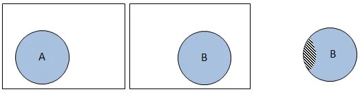
The same is explained in Figure 2.15 using the sample spaces related to the events A and B, assuming that there are few sample points common to these two events. Part 1 of the figure shows the total sample space related to the experiment as in the form of rectangle and the sample space related to the event A as a circle. Similarly part 2 of the figure shows the total sample space and the sample space related to event B. As explained earlier in conditional probability the total sample space is restrained to the sample space that is related to event B (which has already occurred). The same is shown in part 3 of Figure 2.15. Now the sample space for event A (B is the total sample space available) is nothing but the sample points related to event A and falling in the sample space. This is nothing but the intersection of the events A and B and is shown in part 3 of the figure as the hatched area.  

Figure 2.15: Representation of conditional probability using the Venn diagrams

For example, there are 100 trips per day between two places X and Y. Out of these 100 trips 50 are made by car, 25 are made by bus and the other 25 are by local train. Probabilities associated to these modes are 0.5, 0.25, and 0.25, respectively. In transportation engineering both the bus and the local train are considered as public transport so the event space associated to this is the summation of the event spaces associated to bus and local train. Probability of choosing public transportation is 0.5. Now if one is interested in finding the probability of choosing bus given public transportation is chosen the conditional probability is useful in finding that.

Characteristics of Conditional Probability

  • Depends on the Occurrence of Another Event

A key characteristic of conditional probability is that it depends on the occurrence of another event. Unlike simple probability, which measures the likelihood of an event independently, conditional probability considers additional information. The probability of an event changes when another related event has already occurred. For example, the probability of a customer purchasing a printer may increase if the customer has already purchased a laptop. This dependency makes conditional probability highly useful in analyzing real-world situations where events are interconnected and influence one another.

  • Measures Relationships Between Events

Conditional probability helps measure and understand the relationship between two or more events. It shows how the occurrence of one event affects the likelihood of another event occurring. By analyzing these relationships, businesses and researchers can identify patterns and dependencies within data. For example, a retailer may study whether customers who buy one product are more likely to buy another. This characteristic makes conditional probability valuable in market research, risk assessment, and forecasting. It provides insights into event interactions that simple probability cannot capture effectively.

  • Based on Joint Probability

Another important characteristic is that conditional probability relies on joint probability. To calculate conditional probability, the probability of both events occurring together must be known. Joint probability provides the foundation for determining how likely one event is when another has already occurred. This relationship ensures that conditional probability is mathematically consistent and accurate. By using joint probability, analysts can examine event dependencies in a systematic manner. This characteristic highlights the close connection between different probability concepts and their role in statistical analysis.

  • Applicable to Dependent Events

Conditional probability is particularly useful when dealing with dependent events. Dependent events are events where the occurrence of one influences the probability of another. In many business and real-world situations, events are not independent. For example, customer purchasing decisions may depend on previous purchases or promotional offers. Conditional probability helps quantify these dependencies and provides more realistic probability estimates. This characteristic makes it an essential tool for understanding situations where outcomes are interconnected and cannot be analyzed accurately using independent probabilities alone.

  • Provides Updated Probability Estimates

Conditional probability allows probabilities to be updated when new information becomes available. Instead of relying solely on initial estimates, it incorporates additional data to produce revised probability values. This characteristic is especially important in dynamic environments where circumstances change over time. For example, a bank may reassess the probability of loan repayment after receiving updated information about a customer’s financial status. By adjusting probabilities based on current information, conditional probability improves the accuracy and relevance of decision-making and forecasting processes.

  • Supports Better Decision-Making

A significant characteristic of conditional probability is its ability to support informed decision-making. By considering specific conditions and relevant information, it provides more accurate estimates of future outcomes. Managers, investors, and policymakers use conditional probability to evaluate alternatives and assess risks. For example, a business may determine the likelihood of achieving sales targets under certain market conditions. This information enables decision-makers to choose strategies that maximize opportunities and minimize risks. Consequently, conditional probability plays an important role in effective planning and management.

  • Forms the Foundation of Advanced Statistical Methods

Conditional probability serves as the basis for many advanced statistical and analytical techniques. Concepts such as Bayes’ Theorem, predictive modeling, machine learning, and statistical inference all rely on conditional probability principles. By understanding how probabilities change under specific conditions, analysts can develop sophisticated models for forecasting and decision support. This characteristic demonstrates the importance of conditional probability in both theoretical and applied statistics. Its role as a foundational concept makes it essential for advanced research and data analysis across numerous disciplines.

  • Widely Applicable in Real-Life Situations

Conditional probability has broad applicability in business, finance, insurance, healthcare, engineering, and many other fields. Real-world events are often dependent on specific conditions, making conditional probability highly relevant. Businesses use it to analyze customer behavior, assess risks, and forecast demand. Insurance companies use it to estimate claim probabilities based on customer profiles. Financial institutions apply it in credit risk analysis and investment decisions. This widespread applicability demonstrates its practical value and importance. As a result, conditional probability is one of the most widely used concepts in probability and statistics.

Applications of Conditional Probability in Business

  • Customer Purchase Analysis

Conditional probability is widely used to analyze customer purchasing behavior. Businesses calculate the probability that a customer will buy a product given that they have already purchased another related product. For example, a customer who buys a smartphone may also be likely to purchase accessories such as earphones or phone cases. This information helps companies design cross-selling and upselling strategies. By understanding these purchasing relationships, businesses can improve customer experience, increase sales revenue, and develop targeted promotional campaigns. As a result, conditional probability plays a significant role in consumer behavior analysis and marketing decisions.

  • Credit Risk Assessment

Banks and financial institutions use conditional probability to evaluate the likelihood of loan repayment or default under specific conditions. For example, they may calculate the probability that a borrower will default given a low credit score or unstable income. This analysis helps lenders assess creditworthiness and make informed lending decisions. By understanding the relationship between borrower characteristics and repayment behavior, financial institutions can reduce lending risks and improve profitability. Conditional probability therefore serves as an essential tool in credit risk management and financial decision-making.

  • Insurance Underwriting

Insurance companies apply conditional probability to estimate risks associated with policyholders. For example, they may calculate the probability of an accident occurring given a driver’s age, driving history, or vehicle type. These probability estimates help insurers determine premium rates and policy terms. By considering specific conditions, insurance companies can accurately assess risk and avoid financial losses. Conditional probability enables insurers to create fair pricing structures and maintain financial stability. Consequently, it is a critical component of insurance underwriting and risk evaluation processes.

  • Marketing Campaign Evaluation

Businesses use conditional probability to assess the effectiveness of marketing campaigns. They may calculate the probability that a customer makes a purchase after receiving an advertisement or promotional offer. This analysis helps marketers determine which campaigns generate the highest customer response rates. By understanding how promotional activities influence buying behavior, companies can optimize marketing strategies and allocate resources efficiently. Conditional probability also supports customer segmentation and personalized marketing efforts. Therefore, it contributes significantly to improving marketing performance and maximizing returns on investment.

  • Demand Forecasting

Conditional probability plays an important role in demand forecasting by considering specific market conditions. Businesses estimate the probability of future product demand given factors such as seasonal trends, economic conditions, or consumer preferences. This approach provides more accurate demand forecasts than relying solely on historical data. Improved forecasting helps organizations manage inventory, plan production schedules, and allocate resources effectively. By incorporating relevant conditions into predictions, conditional probability reduces uncertainty and enhances operational efficiency. As a result, businesses can better meet customer demand and improve profitability.

  • Quality Control and Production Management

Manufacturing companies use conditional probability to monitor product quality and production efficiency. For example, they may calculate the probability of a product defect occurring given a machine malfunction or a specific production condition. This information helps identify the causes of quality problems and implement corrective measures. By understanding the relationship between production factors and defects, organizations can improve quality standards and reduce waste. Conditional probability therefore supports continuous improvement initiatives and enhances overall manufacturing performance. It is an essential tool for maintaining product reliability and customer satisfaction.

  • Supply Chain and Logistics Management

Conditional probability is valuable in supply chain management because it helps evaluate risks and uncertainties. Businesses may estimate the probability of delayed deliveries given adverse weather conditions, supplier issues, or transportation disruptions. Understanding these probabilities allows organizations to develop contingency plans and improve supply chain resilience. By anticipating potential problems, businesses can reduce operational disruptions and maintain customer service levels. Conditional probability also supports inventory planning and supplier selection. Consequently, it contributes to more efficient and reliable supply chain operations.

  • Investment and Financial Decision-Making

Investors and financial managers use conditional probability to evaluate investment opportunities under specific market conditions. For example, they may calculate the probability of a stock price increase given favorable economic indicators or industry growth. This analysis helps assess investment risks and expected returns. By considering relevant conditions, investors can make more informed decisions and develop effective portfolio strategies. Conditional probability also supports financial forecasting and risk management. Therefore, it plays a crucial role in achieving investment objectives and improving financial performance.

Advantages of Conditional Probability

  • Improves Accuracy of Predictions

One of the major advantages of conditional probability is that it improves the accuracy of predictions by considering additional information. Instead of relying only on general probabilities, it takes into account specific conditions that affect outcomes. For example, a business can estimate future sales based on current market trends and customer behavior. This approach produces more realistic and reliable forecasts. Accurate predictions help organizations reduce uncertainty and make better strategic decisions. As a result, conditional probability is widely used in forecasting, planning, and analytical processes where precise estimates are essential.

  • Supports Better Decision-Making

Conditional probability provides decision-makers with more relevant information by incorporating existing conditions into probability calculations. Managers can evaluate various alternatives and assess the likelihood of different outcomes before making important decisions. For example, a company may determine the probability of a successful product launch given favorable market conditions. This helps in selecting the most effective strategy. By providing a clearer understanding of possible outcomes, conditional probability enables businesses to make informed choices, improve efficiency, and achieve organizational objectives more effectively.

  • Enhances Risk Assessment

Businesses often face risks that depend on specific circumstances. Conditional probability helps assess these risks by measuring the likelihood of an event occurring under particular conditions. For example, banks estimate the probability of loan default based on a borrower’s credit history. This analysis helps organizations identify potential threats and develop risk management strategies. By understanding conditional risks, businesses can take preventive actions and reduce potential losses. Therefore, conditional probability is an important tool for improving risk assessment and ensuring organizational stability.

  • Useful in Customer Behavior Analysis

Conditional probability helps businesses understand customer behavior more effectively. It allows companies to determine the likelihood of a customer taking a specific action given a previous action. For example, a retailer can calculate the probability that a customer purchases accessories after buying a smartphone. Such insights support targeted marketing, personalized recommendations, and cross-selling strategies. Understanding customer behavior enables organizations to improve customer satisfaction and increase sales revenue. Consequently, conditional probability contributes significantly to customer relationship management and marketing effectiveness.

  • Assists in Financial and Investment Planning

Financial institutions and investors use conditional probability to evaluate investment opportunities and financial risks. It helps estimate the probability of favorable returns under specific market conditions. Investors can analyze how economic indicators, interest rates, or industry trends influence investment outcomes. This information supports better portfolio management and resource allocation. By considering relevant conditions, conditional probability improves financial forecasting and investment decision-making. As a result, organizations can maximize returns while minimizing risks, making it an essential tool in financial planning and analysis.

  • Improves Demand Forecasting

Demand forecasting becomes more accurate when businesses consider factors that influence customer demand. Conditional probability allows organizations to estimate future demand based on conditions such as seasonal changes, promotional campaigns, or economic trends. This helps businesses prepare for fluctuations in customer requirements and adjust production accordingly. Accurate demand forecasts reduce inventory costs, prevent stock shortages, and improve operational efficiency. By incorporating relevant information into predictions, conditional probability enhances the reliability of forecasting models and supports effective business planning.

  • Supports Quality Control and Process Improvement

Manufacturing organizations use conditional probability to analyze production quality and identify factors associated with defects. For example, managers can calculate the probability of product defects given specific machine conditions or production processes. This information helps identify root causes of quality issues and implement corrective measures. Improved quality control reduces waste, lowers production costs, and increases customer satisfaction. By supporting continuous process improvement, conditional probability contributes to higher operational efficiency and better product reliability. Therefore, it plays an important role in manufacturing and production management.

  • Widely Applicable Across Different Industries

A significant advantage of conditional probability is its broad applicability. It is used in business, finance, insurance, healthcare, engineering, marketing, and many other fields. Organizations apply it to solve diverse problems involving uncertainty and decision-making. Whether assessing risks, forecasting demand, evaluating investments, or analyzing customer behavior, conditional probability provides valuable insights. Its versatility makes it one of the most important tools in probability and statistics. Because it can be adapted to various situations, conditional probability remains highly relevant in modern business and research environments.

Limitations of Conditional Probability

  • Requires Accurate and Reliable Data

One of the major limitations of conditional probability is its dependence on accurate and reliable data. The probability estimates are only as good as the information used in the calculations. If the data is incomplete, outdated, or incorrect, the resulting probabilities may be misleading. Businesses often face challenges in collecting high-quality data from customers, markets, or operational activities. Poor data quality can lead to inaccurate forecasts and ineffective decisions. Therefore, organizations must invest significant effort in data collection and verification to ensure meaningful and reliable conditional probability analysis.

  • Complex Calculations

Conditional probability calculations can become complicated, especially when multiple variables and conditions are involved. While simple examples are easy to understand, real-world business situations often require advanced statistical methods and large datasets. The complexity increases when there are numerous interrelated events or changing conditions. Managers without statistical expertise may find it difficult to perform or interpret these calculations. As a result, businesses may need specialized software or trained analysts to handle complex probability problems. This complexity can limit the practical application of conditional probability in some situations.

  • Dependent on Assumptions

Many conditional probability models rely on assumptions about the relationships between events. If these assumptions are incorrect, the probability estimates may not accurately reflect reality. For example, analysts may assume that certain factors influence customer behavior in a particular way, even though market conditions may differ. Such assumptions can affect the reliability of the results. In dynamic business environments, relationships between variables may change over time, making earlier assumptions invalid. Therefore, dependence on assumptions is a significant limitation that users must consider when interpreting conditional probability outcomes.

  • Difficult to Interpret

Conditional probability results can sometimes be difficult to interpret, particularly for individuals without a background in statistics. Understanding how one event influences another requires careful analysis and logical reasoning. In complex situations, the meaning of probability values may not be immediately obvious to managers or stakeholders. Misinterpretation can lead to poor decisions and incorrect conclusions. Businesses often need experts to explain and communicate the results effectively. This limitation reduces the accessibility of conditional probability and may create challenges in applying it to everyday business decision-making.

  • Time-Consuming Data Collection

Calculating conditional probability often requires large amounts of detailed information about related events and conditions. Collecting, organizing, and analyzing this data can be time-consuming and resource-intensive. Businesses may need to conduct surveys, monitor transactions, or gather historical records over long periods. This process can delay decision-making and increase operational costs. Small organizations with limited resources may find it particularly challenging to obtain the required information. Consequently, the time and effort involved in data collection can be a significant limitation of conditional probability analysis.

  • Sensitive to Changes in Data

Conditional probability estimates can change significantly when the underlying data changes. Even small variations in the probability of one event may affect the final conditional probability. In rapidly changing business environments, customer preferences, market conditions, and economic factors can alter probability estimates frequently. As a result, previously calculated probabilities may become outdated or less reliable. Businesses must continuously update their data and recalculate probabilities to maintain accuracy. This sensitivity to changing information can increase the complexity and cost of using conditional probability effectively.

  • Limited Predictive Power in Uncertain Situations

Although conditional probability improves prediction accuracy, it cannot guarantee future outcomes. Unexpected events such as economic crises, natural disasters, technological disruptions, or sudden changes in consumer behavior may occur without warning. These unforeseen factors can significantly affect actual results. Conditional probability is based on available information and known relationships, but it cannot account for every possible circumstance. Therefore, its predictive power is limited in highly uncertain or rapidly changing environments. Businesses should use conditional probability as a support tool rather than relying on it exclusively.

  • Cannot Eliminate Uncertainty Completely

Conditional probability helps measure uncertainty, but it cannot remove it entirely. Probability values represent likelihoods rather than certainties. Even when a conditional probability is very high, there is still a chance that the expected event will not occur. Business decisions based solely on probability estimates may overlook qualitative factors such as managerial judgment, market sentiment, or unforeseen opportunities. Therefore, conditional probability should be combined with experience, expertise, and other analytical tools. This limitation reminds decision-makers that uncertainty remains a part of all business activities despite statistical analysis.

Lines of Regression; Co-efficient of regression

Regression Line is the line that best fits the data, such that the overall distance from the line to the points (variable values) plotted on a graph is the smallest. In other words, a line used to minimize the squared deviations of predictions is called as the regression line.

There are as many numbers of regression lines as variables. Suppose we take two variables, say X and Y, then there will be two regression lines:

  • Regression line of Y on X: This gives the most probable values of Y from the given values of X.
  • Regression line of X on Y: This gives the most probable values of X from the given values of Y.

The algebraic expression of these regression lines is called as Regression Equations. There will be two regression equations for the two regression lines.

The correlation between the variables depend on the distance between these two regression lines, such as the nearer the regression lines to each other the higher is the degree of correlation, and the farther the regression lines to each other the lesser is the degree of correlation.

The correlation is said to be either perfect positive or perfect negative when the two regression lines coincide, i.e. only one line exists. In case, the variables are independent; then the correlation will be zero, and the lines of regression will be at right angles, i.e. parallel to the X axis and Y axis.

The regression lines cut each other at the point of average of X and Y. This means, from the point where the lines intersect each other the perpendicular is drawn on the X axis we will get the mean value of X. Similarly, if the horizontal line is drawn on the Y axis we will get the mean value of Y.

Co-efficient of Regression

The Regression Coefficient is the constant ‘b’ in the regression equation that tells about the change in the value of dependent variable corresponding to the unit change in the independent variable.

If there are two regression equations, then there will be two regression coefficients:

  • Regression Coefficient of X on Y:

The regression coefficient of X on Y is represented by the symbol bxy that measures the change in X for the unit change in Y. Symbolically, it can be represented as:

The bxy can be obtained by using the following formula when the deviations are taken from the actual means of X and Y:When the deviations are obtained from the assumed mean, the following formula is used:

  • Regression Coefficient of Y on X:

The symbol byx is used that measures the change in Y corresponding to the unit change in X. Symbolically, it can be represented as:


In case, the deviations are taken from the actual means; the following formula is used:
The byx can be  calculated by using the following formula when the deviations are taken from the assumed means:

The Regression Coefficient is also called as a slope coefficient because it determines the slope of the line i.e. the change in the independent variable for the unit change in the independent variable

Scatter Diagram

Scatter Diagram Method is the simplest method to study the correlation between two variables wherein the values for each pair of a variable is plotted on a graph in the form of dots thereby obtaining as many points as the number of observations. Then by looking at the scatter of several points, the degree of correlation is ascertained.

The degree to which the variables are related to each other depends on the manner in which the points are scattered over the chart. The more the points plotted are scattered over the chart, the lesser is the degree of correlation between the variables. The more the points plotted are closer to the line, the higher is the degree of correlation. The degree of correlation is denoted by “r”.

The following types of scatter diagrams tell about the degree of correlation between variable X and variable Y.

  1. Perfect Positive Correlation (r = +1):

The correlation is said to be perfectly positive when all the points lie on the straight line rising from the lower left-hand corner to the upper right-hand corner.

2. Perfect Negative Correlation (r = -1):

When all the points lie on a straight line falling from the upper left-hand corner to the lower right-hand corner, the variables are said to be negatively correlated.

3. High Degree of +Ve Correlation (r = + High):

The degree of correlation is high when the points plotted fall under the narrow band and is said to be positive when these show the rising tendency from the lower left-hand corner to the upper right-hand corner.

4. High Degree of –Ve Correlation (r = – High):

The degree of negative correlation is high when the point plotted fall in the narrow band and show the declining tendency from the upper left-hand corner to the lower right-hand corner.

5. Low degree of +Ve Correlation (r = + Low):

The correlation between the variables is said to be low but positive when the points are highly scattered over the graph and show a rising tendency from the lower left-hand corner to the upper right-hand corner.

6. Low Degree of –Ve Correlation (r = + Low):

The degree of correlation is low and negative when the points are scattered over the graph and the show the falling tendency from the upper left-hand corner to the lower right-hand corner.

7. No Correlation (r = 0):

The variable is said to be unrelated when the points are haphazardly scattered over the graph and do not show any specific pattern. Here the correlation is absent and hence r = 0.

Thus, the scatter diagram method is the simplest device to study the degree of relationship between the variables by plotting the dots for each pair of variable values given. The chart on which the dots are plotted is also called as a Dotogram.

Mean Deviation, Coefficient of Mean Deviation and Standard Deviation

Mean Deviation

Mean deviation is a measure of dispersion that indicates the average of the absolute differences between each data point and the mean (or median) of the dataset. It provides an overall sense of how much the values deviate from the central value. To calculate mean deviation, the absolute differences between each data point and the central measure are summed and then divided by the number of observations. Unlike variance, mean deviation is expressed in the same units as the data and is less sensitive to extreme outliers.

The basic formula for finding out mean deviation is :

Mean Deviation = Sum of absolute values of deviations from ‘a’ ÷ The number of observations

Coefficient of Mean Deviation

Coefficient of Mean Deviation is a relative measure of dispersion that expresses the Mean Deviation in relation to the average from which the deviations are calculated. It is useful for comparing the variability of different datasets, especially when their units or average values are different.

Formula: Coefficient of Mean Deviation = Mean Deviation / Average

The average may be Arithmetic Mean, Median, or Mode, depending on the basis used for calculating Mean Deviation.

If Mean Deviation is calculated from the Mean:

Coefficient of M.D.= MDXˉ / Xˉ

If it is calculated from the Median:

Example

Suppose the Mean Deviation = 8 and the Mean = 40.

Coefficient of M.D.= 8 / 40 = 0.20

Therefore, the Coefficient of Mean Deviation = 0.20.

If expressed as a percentage:

0.20 × 100 = 20%

Computation of Mean Deviation

1. Meaning and Concept of Mean Deviation

Mean Deviation (MD) is an absolute measure of dispersion that indicates the average amount by which observations differ from a central value. The central value may be the Arithmetic Mean, Median, or Mode. While calculating Mean Deviation, positive and negative signs are ignored by taking absolute deviations. It helps determine the degree of variation and consistency in a dataset. A lower Mean Deviation indicates greater concentration around the selected average.

2. Computation for Individual Series

For an Individual Series, Mean Deviation is calculated by taking the absolute difference between every observation and the selected average. The absolute deviations are then added and divided by the total number of observations. The formula is: MD = Σ|X − A| / N. Here, X represents an observation, A represents Mean, Median, or Mode, and N represents the number of observations. This method is suitable when observations are given separately.

3. Computation for Discrete Series

In a Discrete Series, each variable has a corresponding frequency. First, the selected average is calculated. Then, the absolute deviation of every value from that average is determined and multiplied by its frequency. The products are added and divided by total frequency. The formula is: MD = Σf|X − A| / Σf. Here, f represents frequency, X represents the value, and A represents the selected average used for calculating Mean Deviation.

4. Computation for Continuous Series

For a Continuous Series, Mean Deviation is calculated using the midpoints of class intervals. First, the midpoint of every class is determined and treated as X. The absolute deviation from the selected average is then calculated and multiplied by frequency. The total of these products is divided by total frequency. The formula is: MD = Σf|X − A| / Σf. This method is useful for analysing data presented through continuous class intervals.

5. Selection of Central Value

Mean Deviation can be calculated from the Mean, Median, or Mode. The choice depends upon the nature of the data and the purpose of analysis. Generally, the Median is preferred because Mean Deviation calculated from the Median is minimum compared with other central values. The selected average provides the reference point from which absolute deviations are measured. Therefore, proper selection of the central value is important for meaningful results.

6. Steps in Computation

The computation of Mean Deviation involves several systematic steps. First, identify the appropriate central value. Second, calculate the deviation of each observation from that value. Third, ignore the positive and negative signs by taking absolute values. Fourth, multiply deviations by frequencies for discrete or continuous series. Fifth, add the resulting values and divide by the total number of observations or frequency. This procedure produces the required Mean Deviation.

7. Coefficient of Mean Deviation

The Coefficient of Mean Deviation is a relative measure used to compare the dispersion of different datasets. It is obtained by dividing Mean Deviation by the central value from which the deviation was calculated. The formula is: Coefficient of M.D. = Mean Deviation / Average. If Median is used, the formula becomes Coefficient of M.D. = M.D. / Median. A lower coefficient indicates greater consistency, while a higher coefficient indicates greater relative variability.

8. Interpretation of Mean Deviation

Mean Deviation indicates the average distance of observations from a selected central value. A low Mean Deviation means that observations are closely concentrated around the average, showing greater consistency. A high Mean Deviation indicates that observations are widely dispersed and less consistent. Therefore, Mean Deviation provides a simple numerical measure of variability. It is useful for understanding the extent to which observations differ from their central tendency.

Applications of Mean Deviation

1. Business Performance Analysis

Mean Deviation is useful in analysing variations in sales, production, revenue, costs, and profits. It helps managers determine how far individual business results generally differ from the average performance. A smaller Mean Deviation indicates greater stability and consistency, whereas a larger value indicates greater fluctuations. This information can support managerial planning, performance evaluation, budgeting, and control. Therefore, Mean Deviation provides a useful measure for understanding variability in different areas of business operations.

2. Financial Analysis

In financial analysis, Mean Deviation can be used to study variations in income, expenditure, returns, prices, and other financial variables. It indicates the average extent to which financial observations differ from their selected central value. This helps analysts understand the consistency of financial performance. By examining dispersion along with central tendency, financial managers can make more informed decisions regarding planning, budgeting, investment evaluation, and financial control.

3. Wage and Income Analysis

Mean Deviation is useful for studying variations in wages, salaries, and incomes among individuals or groups. It indicates how far individual earnings generally differ from the average or median income. A lower Mean Deviation suggests greater uniformity in earnings, while a higher value indicates greater inequality or variation. Governments, researchers, and organizations can use this information to study income patterns and understand the distribution of earnings within a population.

4. Educational Analysis

Educational institutions can apply Mean Deviation to analyse variations in marks, grades, attendance, and academic performance. It helps determine how closely students’ results are concentrated around the average performance. A low Mean Deviation indicates relatively consistent performance, whereas a high value indicates substantial differences among students. Teachers and administrators can use this information to evaluate academic patterns, identify variations in achievement, and support educational planning and improvement.

5. Market Research

Mean Deviation has important applications in market research for studying variations in customer spending, product demand, sales, prices, and purchasing behaviour. It helps researchers determine the average extent of variation around a selected central value. Understanding dispersion enables businesses to identify whether consumer behaviour is relatively stable or highly variable. Such information can support decisions related to pricing, production, marketing strategies, inventory management, and sales forecasting.

6. Quality Control

In quality control, Mean Deviation helps measure variations in product characteristics such as weight, size, dimensions, quantity, and production output. It indicates how far individual measurements differ from the selected standard or central value. A smaller Mean Deviation generally indicates greater consistency in production, while a larger value may suggest greater variation. Therefore, it can help manufacturers monitor production quality, identify inconsistencies, and improve manufacturing processes.

7. Economic Analysis

Mean Deviation is useful in economic analysis for studying variations in prices, income, consumption, production, employment, and other economic variables. It provides information about the degree of dispersion around a central value. Economists can use it to understand the stability or variability of economic conditions. When combined with measures of central tendency, Mean Deviation provides a clearer picture of the distribution and consistency of economic data.

8. Comparison of Data

Mean Deviation and its coefficient can be used to compare the variability of different datasets. Absolute Mean Deviation is useful when datasets are expressed in similar units, while the Coefficient of Mean Deviation is more suitable when their magnitudes or averages differ. A lower coefficient generally indicates greater consistency, whereas a higher coefficient indicates greater relative dispersion. Thus, Mean Deviation supports meaningful comparison between different groups or distributions.

Advantages

  • It is a relative measure of dispersion.
  • It facilitates comparison between different distributions.
  • It is simple to calculate and understand.
  • It is based on absolute deviations.
  • It can be calculated using Mean or Median.
  • It is useful when datasets have different magnitudes.
  • It provides a standardized measure of variability.
  • It is useful in business and economic analysis.

Limitations

  • It is not based on algebraic deviations.
  • It is less useful for advanced mathematical analysis.
  • Its value depends on the average selected.
  • It gives less importance to extreme values than standard deviation.
  • It may not be suitable for all types of statistical analysis.
  • Calculation can become lengthy for large datasets.
  • It does not use the squared deviations used in standard deviation.
  • It is less widely used than the Coefficient of Variation.

Standard Deviation

Standard deviation is a widely used measure of dispersion that indicates the average amount by which each data point deviates from the mean. It is calculated by first finding the variance, which is the average of squared deviations, and then taking the square root of the variance. Standard deviation provides a more interpretable measure of spread, as it is in the same units as the original data. A higher standard deviation indicates greater variability, while a lower value indicates data points are closer to the mean, indicating less spread or consistency.

Usually represented by s or σ. It uses the arithmetic mean of the distribution as the reference point and normalizes the deviation of all the data values from this mean.

Therefore, we define the formula for the standard deviation of the distribution of a variable X with n data points as:

Combined Standard Deviation

Combined Standard Deviation is a statistical measure used to determine the standard deviation of two or more groups taken together. It considers the number of observations, individual standard deviations, and differences between group means. It provides a single measure of dispersion for the combined data and is useful when separate groups need to be analysed as one population.

Formula: Combined S.D. = √[N₁(σ₁² + d₁²) + N₂(σ₂² + d₂²)] / √(N₁ + N₂)

Where:

N₁, N₂ = Number of observations in the groups
σ₁, σ₂ = Standard deviations of the groups
d₁, d₂ = Differences between group means and combined mean

Combined Mean

Combined Mean = (N₁X̄₁ + N₂X̄₂) / (N₁ + N₂)

Computation of Standard Deviation

1. Meaning and Concept of Standard Deviation

Standard Deviation (SD) is an important absolute measure of dispersion that shows the extent to which observations differ from their Arithmetic Mean. It is calculated by taking the square root of the average of the squared deviations from the mean. A smaller Standard Deviation indicates greater consistency, while a larger value indicates greater variability. It is widely used because it considers all observations and provides a reliable measure of dispersion.

2. Computation for Individual Series

For an Individual Series, Standard Deviation is calculated by first finding the Arithmetic Mean. The deviation of each observation from the mean is then calculated and squared. These squared deviations are added and divided by the total number of observations. Finally, the square root of the result is taken. Formula: SD = √[Σ(X − X̄)² / N]. Here, X represents observations, X̄ represents the mean, and N represents observations.

3. Computation for Discrete Series

In a Discrete Series, each value is associated with a frequency. First, the Arithmetic Mean is calculated. Then, deviations of each value from the mean are obtained and squared. Each squared deviation is multiplied by its corresponding frequency. The total is divided by the total frequency, and the square root is taken. Formula: SD = √[Σf(X − X̄)² / Σf]. This method considers both values and their respective frequencies.

4. Computation for Continuous Series

For a Continuous Series, Standard Deviation is calculated using the midpoints of class intervals. The midpoint represents each class and is treated as X. Deviations from the Arithmetic Mean are calculated and squared, then multiplied by the corresponding frequencies. The sum is divided by total frequency, followed by taking the square root. Formula: SD = √[Σf(X − X̄)² / Σf]. This method is suitable for grouped continuous data.

5. Direct Method

The Direct Method calculates Standard Deviation by using the actual deviations of observations from the Arithmetic Mean. The formula for an individual series is SD = √[Σ(X − X̄)² / N]. For frequency distributions, frequencies are incorporated into the calculation. Although this method is conceptually simple, it can become lengthy when observations are large or contain inconvenient numerical values. It is mainly useful when the Arithmetic Mean is easy to calculate.

6. Assumed Mean Method

Assumed Mean Method simplifies the calculation when the actual mean is inconvenient to use. A convenient value is selected as the Assumed Mean (A), and deviations are calculated from it. The formula is: SD = √[(Σd² / N) − (Σd / N)²], where d represents deviation from the assumed mean. This method reduces calculation work and is particularly useful for datasets containing large values.

7. Step-Deviation Method

Step-Deviation Method is a simplified form of the assumed mean method, especially useful when class intervals have a common width. Deviations are divided by the common class interval. The formula is: SD = i√[(Σfu² / Σf) − (Σfu / Σf)²]. Here, i represents the common class interval and u represents step-deviations. This method considerably reduces the size of calculations in large frequency distributions.

8. Interpretation of Standard Deviation

Standard Deviation measures the overall spread of observations around the mean. A low Standard Deviation indicates that observations are closely concentrated around the mean, showing greater consistency. A high Standard Deviation indicates greater dispersion and less consistency. Since it is expressed in the same units as the original observations, it is easy to interpret. Standard Deviation also forms the basis for several advanced statistical techniques.

Applications of Standard Deviation

1. Business Performance Analysis

Standard Deviation is widely used in business analysis to measure variations in sales, production, revenue, costs, and profits. It helps managers determine the stability of business performance. A low Standard Deviation indicates consistent results, while a high value indicates significant fluctuations. This information can support planning, budgeting, performance evaluation, and managerial decision-making. Therefore, Standard Deviation provides a reliable measure for analysing variability in different business activities.

2. Financial and Investment Analysis

In financial analysis, Standard Deviation is commonly used to measure the variability of investment returns. A higher Standard Deviation generally indicates greater fluctuation in returns and therefore greater investment risk. Investors can use it to compare the stability of different investments and evaluate risk-return characteristics. It is also useful in portfolio analysis, financial planning, and assessment of market performance where variation in returns is an important consideration.

3. Quality Control

Standard Deviation is an important tool in quality control because it measures variation in production processes. It can be used to study differences in product weight, size, dimensions, strength, or other characteristics. A small Standard Deviation indicates that products are produced consistently, while a large value suggests greater variation. Manufacturers can use this information to identify production problems, maintain quality standards, and improve operational efficiency.

4. Educational Analysis

In education, Standard Deviation is used to analyse variations in students’ marks, grades, test scores, and academic performance. It helps determine whether students’ results are concentrated around the average or widely dispersed. A low Standard Deviation suggests relatively similar performance, while a high value indicates greater differences among students. Educational institutions can use this information for performance evaluation, examination analysis, and comparison of academic results.

5. Economic Analysis

Standard Deviation is useful in economic studies for analysing variations in income, prices, employment, production, consumption, and other economic variables. It helps economists understand the stability and distribution of economic data. By studying Standard Deviation along with measures of central tendency, researchers can obtain a better understanding of economic conditions. It is particularly useful when comparing variability across different periods, regions, or economic groups.

6. Market Research

In market research, Standard Deviation helps measure variations in customer spending, product demand, sales, prices, and consumer preferences. It enables businesses to determine whether market behaviour is relatively stable or highly variable. A lower Standard Deviation indicates greater consistency in observations, while a higher value suggests greater variation. This information can assist businesses in marketing planning, pricing decisions, demand analysis, and sales forecasting.

7. Scientific and Research Analysis

Standard Deviation is widely applied in scientific research to measure the variability of experimental observations. Researchers use it to determine how closely observations are distributed around their mean. It helps assess the consistency and reliability of experimental results. Standard Deviation is also an important component of many statistical techniques, including correlation, regression, hypothesis testing, and statistical estimation, making it essential for quantitative research.

8. Comparison and Decision-Making

Standard Deviation provides a useful basis for comparison and decision-making. When datasets are measured in the same units, their Standard Deviations can be compared directly to determine which has greater variability. When combined with the Coefficient of Variation, it can also help compare relative consistency between datasets with different averages. Therefore, Standard Deviation supports effective decisions in business, finance, economics, education, research, and other fields.

Median Characteristics, Applications and Limitations

Median is a measure of central tendency that represents the middle value of an ordered dataset, dividing it into two equal halves. If the dataset has an odd number of values, the median is the middle value. If the dataset has an even number, it is the average of the two middle values. The median is less affected by outliers, making it useful for skewed data or non-uniform distributions.

Example:

The marks of nine students in a geography test that had a maximum possible mark of 50 are given below:

     47     35     37     32     38     39     36     34     35

Find the median of this set of data values.

Solution:

Arrange the data values in order from the lowest value to the highest value:

    32     34     35     35     36     37     38     39     47

The fifth data value, 36, is the middle value in this arrangement.

Characteristics of Median:

  1. Middle Value of Data

The median divides a dataset into two equal halves, with 50% of the values lying below it and 50% above it. It is determined by arranging data in ascending or descending order.

  1. Resistant to Outliers

The median is not influenced by extreme values or outliers. This makes it a more robust measure for datasets with significant variability or skewness.

  1. Applicable to Ordinal and Quantitative Data

The median can be calculated for ordinal data (where data can be ranked) and quantitative data. It is not suitable for nominal data, as there is no inherent order.

  1. Unique Value

For any given dataset, the median is always unique and provides a single central value, ensuring consistency in its interpretation.

  1. Requires Data Sorting

The calculation of the median necessitates ordering the data values. Without arranging the data, the median cannot be identified.

  1. Effective for Skewed Distributions

In skewed datasets, the median better represents the center compared to the mean, as it remains unaffected by the skewness.

  1. Not Affected by Sample Size

Median’s calculation is straightforward and remains valid regardless of the sample size, as long as the data is properly ordered.

Applications of Median:

  1. Income and Wealth Distribution

In economics and social studies, the median is used to analyze income and wealth distributions. For example, the median income indicates the income level at which half the population earns less and half earns more. It is more accurate than the mean in scenarios with extreme disparities, such as high-income earners skewing the average.

  1. Real Estate Market Analysis

Median is commonly applied in the real estate industry to determine the central value of property prices. Median house prices are preferred over averages because they are less affected by outliers, such as extremely high or low-priced properties.

  1. Educational Assessments

In education, the median is used to evaluate student performance. For example, the median test score helps identify the middle-performing student, providing a fair representation when the scores are unevenly distributed.

  1. Medical and Health Statistics

Median is often employed in health sciences to summarize data such as median survival rates or recovery times. These metrics are crucial when the data includes extreme cases or a non-symmetric distribution.

  1. Demographic Studies

Median age, household size, and other demographic measures are widely used in population studies. These metrics provide insights into the central characteristics of populations while avoiding distortion by extremes.

  1. Transportation Planning

In transportation and traffic analysis, the median is used to determine the typical travel time or commute duration. It offers a realistic measure when the data includes unusually long or short travel times.

Demerits or Limitations of Median:

  1. Even if the value of extreme items is too large, it does not affect too much, but due to this reason, sometimes median does not remain the representative of the series.
  2. It is affected much more by fluctuations of sampling than A.M.
  3. Median cannot be used for further algebraic treatment. Unlike mean we can neither find total of terms as in case of A.M. nor median of some groups when combined.
  4. In a continuous series it has to be interpolated. We can find its true-value only if the frequencies are uniformly spread over the whole class interval in which median lies.
  5. If the number of series is even, we can only make its estimate; as the A.M. of two middle terms is taken as Median.

error: Content is protected !!