Causation Method

Causal inference is the process of drawing a conclusion about a causal connection based on the conditions of the occurrence of an effect. The main difference between causal inference and inference of association is that the former analyzes the response of the effect variable when the cause is changed. The science of why things occur is called etiology. Causal inference is an example of causal reasoning.

In statistics, causation is a bit tricky. As you’ve no doubt heard, correlation doesn’t necessarily imply causation. An association or correlation between variables simply indicates that the values vary together. It does not necessarily suggest that changes in one variable cause changes in the other variable. Proving causality can be difficult.

Relationships and Correlation

The expression is, “correlation does not imply causation.” Consequently, you might think that it applies to things like Pearson’s correlation coefficient. And, it does apply to that statistic. However, we’re really talking about relationships between variables in a broader context. Pearson’s is for two continuous variables. However, a relationship can involve different types of variables such as categorical variables, counts, binary data, and so on.

For example, in a medical experiment, you might have a categorical variable that defines which treatment group subjects belong to control group, placebo group, and several different treatment groups. If the health outcome is a continuous variable, you can assess the differences between group means. If the means differ by group, then you can say that mean health outcomes depend on the treatment group. There’s a correlation, or relationship, between the type of treatment and health outcome. Or, maybe we have the treatment groups and the outcome is binary, say infected and not infected. In that case, we’d compare group proportions of the infected/not infected between groups to determine whether treatment correlates with infection rates.

Through this post, I’ll refer to correlation and relationships in this broader sense not just literal correlation coefficients. But relationships between variables, such as differences between group means and proportions, regression coefficients, associations between pairs of categorical variables, and so on.

Causation and Hypothesis Tests

Before moving on to determining whether a relationship is causal, let’s take a moment to reflect on why statistically significant hypothesis test results do not signify causation.

Hypothesis tests are inferential procedures. They allow you to use relatively small samples to draw conclusions about entire populations. For the topic of causation, we need to understand what statistical significance means.

When you see a relationship in sample data, whether it is a correlation coefficient, a difference between group means, or a regression coefficient, hypothesis tests help you determine whether your sample provides sufficient evidence to conclude that the relationship exists in the population. You can see it in your sample, but you need to know whether it exists in the population. It’s possible that random sampling error (i.e., luck of the draw) produced the “relationship” in your sample.

Statistical significance indicates that you have sufficient evidence to conclude that the relationship you observe in the sample also exists in the population.

Hill’s Criteria of Causation

Determining whether a causal relationship exists requires far more in-depth subject area knowledge and contextual information than you can include in a hypothesis test. In 1965, Austin Hill, a medical statistician, tackled this question in a paper that’s become the standard. While he introduced it in the context of epidemiological research, you can apply the ideas to other fields.

Hill describes nine criteria to help establish causal connections. The goal is to satisfy as many criteria possible. No single criterion is sufficient. However, it’s often impossible to meet all the criteria. These criteria are an exercise in critical thought. They show you how to think about determining causation and highlight essential qualities to consider.

Correlation mean causation

Even if there is a correlation between two variables, we cannot conclude that one variable causes a change in the other. This relationship could be coincidental, or a third factor may be causing both variables to change.

For example, Ankit collected data on the sales of ice cream cones and air conditioners in his hometown. He found that when ice cream sales were low, air conditioner sales tended to be low and that when ice cream sales were high, air conditioner sales tended to be high.

  • Ankit can conclude that sales of ice cream cones and air conditioner are positively correlated.
  • Ankit can’t conclude that selling more ice cream cones causes more air conditioners to be sold. It is likely that the increases in the sales of both ice cream cones and air conditioners are caused by a third factor, an increase in temperature!

Concurrent Deviation Method

The method of studying correlation is the simplest of all the methods. The only thing that is required under this method is to find out the direction of change of X variable and Y variable.

A very simple and casual method of finding correlation when we are not serious about the magnitude of the two variables is the application of concurrent deviations.

This method involves in attaching a positive sign for a x-value (except the first) if this value is more than the previous value and assigning a negative value if this value is less than the previous value.

This is done for the y-series as well. The deviation in the x-value and the corresponding y-value is known to be concurrent if both the deviations have the same sign.

Denoting the number of concurrent deviations by c and total number of deviations as m (which must be one less than the number of pairs of x and y values), the coefficient of concurrent-deviations is given by 

rc = +√+ (2C-n)/n

Where rc stands for coefficient of correlation by the concurrent deviation method; C stands for

the number of concurrent deviations or the number of positive signs obtained after multiplying

Dx with Dy

n = Number of pairs of observations compared.

Steps

(i) find out the direction of change of X variable, i.e., as compared with the first value, whether the second value is increasing or decreasing or is constant. If it is increasing put (+) sign; if it is decreasing put (-) sign (minus) and if it is constant put zero. Similarly, as compared to second value find out whether the third value is increasing, decreasing or constant. Repeat the same process for other values. Denote this column by Dx.

(ii) In the same manner as discussed above find out the direction of change of Y variable and denote this column by Dy.

(iii) Multiply Dx with Dy, and determine the value of c, i.e., the number of positive signs.

(iv) Apply the above formula, i.e.,

rc = +√+ (2C-n)/n

Note. The significance of + signs, both (inside the under root and outside the under root) is that we cannot take the under root of minus sign. Therefore, if 2C – n   is negative, this negative  

value of multiplied with the minus sign inside would make it positive and we can take the under root. But the ultimate result would be negative. If 2C-n  is positive then, of course, we get a positive value of the coefficient of correlation.

Percentiles

Percentile is in everyday use, but there is no universal definition for it. The most common definition of a percentile is a number where a certain percentage of scores fall below that number. You might know that you scored 67 out of 90 on a test. But that figure has no real meaning unless you know what percentile you fall into. If you know that your score is in the 90th percentile, that means you scored better than 90% of people who took the test.

In statistics, a percentile (or a centile) is a score below which a given percentage of scores in its frequency distribution fall (exclusive definition) or a score at or below which a given percentage fall (inclusive definition). For example, the 50th percentile (the median) is the score below which 50% (exclusive) or at or below which (inclusive) 50% of the scores in the distribution may be found.

The percentile (or percentile score) and the percentile rank are related terms. The percentile rank of a score is the percentage of scores in its distribution that are less than it, an exclusive definition, and one that can be expressed with a single, simple formula. In contrast, there is not one formula or algorithm for a percentile score but many. Hyndman and Fan identified nine and most statistical and spreadsheet software use one of the methods they describe. Algorithms either return the value of a score that exists in the set of scores (nearest-rank methods) or interpolate between existing scores and are either exclusive or inclusive.

  • The 25th percentile is also called the first quartile.
  • The 50th percentile is generally the median.
  • The 75th percentile is also called the third quartile.
  • The difference between the third and first quartiles is the interquartile range.

Simple and Weighted Averages

Simple Averages

Simple average of a set of values is determined by dividing the sum total of all the values by the number of values in the set.

The formula of simple average can be expressed as follows:

Simple average = (Total of x1 + x2+x3…..+xn)/n

Where;

    x = values in the set

    n = number of values in the set

Weighted average

Weighted average is a means of determining the average of a set of values by assigning weightage to each value in relation to their relative importance/significance.

The formula of weighted average can be expressed as follows:

Weighted average = (Total of x1w1+ x2w2+x3w3…..+xnwn)/(Total of w1 +w2+w3….+wn)

Where;

    x = values in the set

    w = weightage of each value in the set

    n = number of values in the set

Graphic presentation: Technique of Construction of Graphs

Graphic presentation represents a highly developed body of techniques for elucidating, interpreting, and analyzing numerical facts by means of points, lines, areas, and other geometric forms and symbols. Graphic techniques are especially valuable in presenting quantitative data in a simple, clear, and effective manner, as well as facilitating comparisons of values, trends, and relationships. They have the additional advantages of succinctness and popular appeal; the comprehensive pictures they provide can bring out hidden facts and relationships and contribute to a more balanced understanding of a problem.

The choice of a particular graphic technique to present a given set of data is a difficult one, and no hard and fast rules can be made to cover all circumstances. There are, however, certain general goals that should always be kept in mind. These include completeness, clarity, and honesty; but there is often conflict between the goals. For instance, completeness demands that all data points be included in a chart, but often this can be done only at some sacrifice of clarity. Such problems can be mitigated by the practice (highly desirable on other grounds as well) of indicating the source of the data from which the chart was constructed so that the reader himself can investigate further. Another problem occurs when it is necessary to break an axis in order to fit all the data in a reasonable space; clarity is then served, but honesty demands that attention be strongly called to the break.

On the basis of form, charts and graphs may be classified as:

(1) Rectilinear coordinate graphs

(2) Semilogarithmic charts

(3) Bar and column charts

(4) Frequency graphs and related charts

(5) Maps

(6) Miscellaneous charts, including pie diagrams, scattergrams, fan charts, ranking charts, etc.

(7) Pictorial charts

(8) Three-dimensional projection charts.

General Rules for Graphical Representation of Data

There are certain rules to effectively present the information in the graphical representation. They are:

  • Suitable Title: Make sure that the appropriate title is given to the graph which indicates the subject of the presentation.
  • Measurement Unit: Mention the measurement unit in the graph.
  • Proper Scale: To represent the data in an accurate manner, choose a proper scale.
  • Index: Index the appropriate colours, shades, lines, design in the graphs for better understanding.
  • Data Sources: Include the source of information wherever it is necessary at the bottom of the graph.
  • Keep it Simple: Construct a graph in an easy way that everyone can understand.
  • Neat: Choose the correct size, fonts, colours etc. in such a way that the graph should be a visual aid for the presentation of information.

Construction of a Graph

The graphic presentation of data and information offers a quick and simple way of understanding the features and drawing comparisons. Further, it is an effective analytical tool and a graph can help us in finding the mode, median, etc.

One can locate a point in a plane using two mutually perpendicular lines – the X-axis (the horizontal line) and the Y-axis (the vertical line). Their point of intersection is the Origin.

One can locate the position of a point in terms of its distance from both these axes. For example, if a point P is 3 units away from the Y-axis and 5 units away from the X-axis, then its location is as follows:

Key Points

  • We measure the distance of the point from the Y-axis along the X-axis. Similarly, we measure the distance of the point from the X-axis along the Y-axis. Therefore, to measure 3 units from the Y-axis, we move 3 units along the X-axis and likewise for the other coordinate.
  • We then draw perpendicular lines from these two points.
  • The point where the perpendiculars intersect is the position of the point P.
  • We denote it as follows (3,5) or (abscissa, ordinate). Together, they are the coordinates of the point P.
  • The four parts of the plane are Quadrants.
  • Also, we can plot different points for a different pair of values.

Graphs of Frequency Distribution

Frequency distribution, in statistics, a graph or data set organized to show the frequency of occurrence of each possible outcome of a repeatable event observed many times. Simple examples are election returns and test scores listed by percentile. A frequency distribution can be graphed as a histogram or pie chart. For large data sets, the stepped graph of a histogram is often approximated by the smooth curve of a distribution function (called a density function when normalized so that the area under the curve.

In statistics, a frequency distribution is a list, table or graph that displays the frequency of various outcomes in a sample. Each entry in the table contains the frequency or count of the occurrences of values within a particular group or interval.

The famed bell curve, or normal distribution, is the graph of one such function. Frequency distributions are particularly useful in summarizing large data sets and assigning probabilities.

Applications

Managing and operating on frequency tabulated data is much simpler than operation on raw data. There are simple algorithms to calculate median, mean, standard deviation etc. from these tables.

Statistical hypothesis testing is founded on the assessment of differences and similarities between frequency distributions. This assessment involves measures of central tendency or averages, such as the mean and median, and measures of variability or statistical dispersion, such as the standard deviation or variance.

A frequency distribution is said to be skewed when its mean and median are significantly different, or more generally when it is asymmetric. The kurtosis of a frequency distribution is a measure of the proportion of extreme values (outliers), which appear at either end of the histogram. If the distribution is more outlier-prone than the normal distribution it is said to be leptokurtic; if less outlier-prone it is said to be platykurtic.

Letter frequency distributions are also used in frequency analysis to crack ciphers, and are used to compare the relative frequencies of letters in different languages and other languages are often used like Greek, Latin, etc.

Types of Frequency Distribution

  • Grouped frequency distribution.
  • Ungrouped frequency distribution.
  • Cumulative frequency distribution.
  • Relative frequency distribution.
  • Relative cumulative frequency distribution.

Grouped Data

At certain times to ensure that we are making correct and relevant observations from the data set, we may need to group the data into class intervals. This ensures that the frequency distribution best represents the data. Let us make a grouped frequency data table of the same example above of the height of students.

Class IntervalFrequency
130-1404
140-1505
150-1603

From the above table, you can see that the value of 150 is put in the class interval of 150-160 and not 140-150.

Example

Frequency Distribution Table

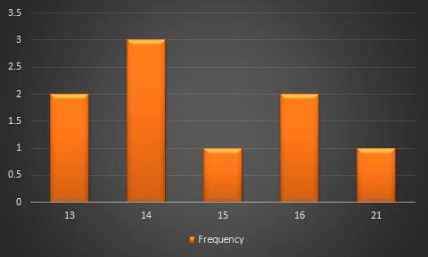
13,14,16,13,16,14,21,14,15

HeightFrequency
132
143
151
162
211

Diagrammatic Presentation of Data, One Dimensional and Two-Dimensional Diagrams

Diagrammatic Presentation of Data refers to the method of presenting statistical information through diagrams, charts, and visual forms. It converts numerical data into an attractive and easily understandable form. Diagrams are especially useful when information needs to be communicated to people who may not be familiar with detailed statistical tables. They help in making comparisons, identifying trends, understanding proportions, and highlighting important features of data. Diagrammatic presentation is widely used in business reports, newspapers, research studies, government publications, and presentations.

1. Simple Bar Diagram

Simple Bar Diagram represents data using rectangular bars of equal width, where the length or height of each bar is proportional to the value being represented. Bars are generally separated by equal spaces and can be drawn vertically or horizontally. It is mainly used for comparing different categories of data. The categories are shown on one axis and their corresponding values on the other axis. Example: A company may represent annual sales of four products as Product A – ₹20 lakh, Product B – ₹30 lakh, Product C – ₹25 lakh, and Product D – ₹40 lakh. The tallest bar will represent Product D. Simple bar diagrams make comparisons quick, clear, and visually understandable.

2. Multiple Bar Diagram

Multiple Bar Diagram is used when two or more related sets of data need to be compared simultaneously. In this diagram, several bars are placed together for each category, with each bar representing a different variable. Different patterns, shades, or colours may be used to distinguish the variables. It is useful for comparing changes between related groups. Example: A company may compare the sales of Products A and B during three years. For each year, two bars can be drawn side by side—one for Product A and another for Product B. Multiple bar diagrams allow users to observe differences and relationships between several datasets conveniently and clearly.

3. Component Bar Diagram

Component Bar Diagram represents a total quantity through a single bar that is divided into different components or parts. Each component is proportional to its contribution to the total. It is useful for showing both the total value and the composition of that total. Example: A company’s total expenditure of ₹10 lakh may consist of salaries ₹4 lakh, raw materials ₹3 lakh, transportation ₹2 lakh, and other expenses ₹1 lakh. A single bar representing ₹10 lakh can be divided into these four components. Component bar diagrams help users understand how a total amount is distributed among different parts and are particularly useful for analysing the composition of business expenditure, income, production, or population.

4. Percentage Bar Diagram

Percentage Bar Diagram presents each total quantity as a bar divided into components according to their percentage contribution. Every bar represents 100 percent, regardless of the actual total value. This makes it particularly useful for comparing the relative composition of different groups. Example: Suppose the expenditure of a family consists of 40% food, 25% housing, 20% education, and 15% transport. A bar representing 100% can be divided into these four sections. If expenditure patterns for different families or years are compared, percentage bars make differences in composition easy to identify. Thus, percentage bar diagrams are useful when the objective is to compare proportions or relative shares rather than absolute quantities.

5. Pie Diagram

Pie Diagram, also called a Pie Chart, is a circular diagram divided into sectors representing different components of a total. The complete circle represents 100% or 360°, and the angle of each sector is proportional to its corresponding value. The angle can be calculated using the formula: Angle = Value ÷ Total × 360°. Example: If a company’s total expenditure is divided into salaries 40%, materials 30%, rent 20%, and other expenses 10%, the circle can be divided into sectors representing these percentages. Pie diagrams are particularly useful for showing the composition and relative importance of different components within a total.

6. Pictogram

Pictogram presents statistical information using pictures, symbols, or icons, where each picture represents a specific numerical quantity. It is a simple and attractive method of presenting data and is especially suitable for general audiences and elementary statistical communication. A key or legend is provided to explain the value represented by each symbol. Example: If one book symbol represents 100 books sold, then five symbols represent 500 books sold. A pictogram can be used to display the sales of different products, number of students, or production levels. Although it is visually appealing and easy to understand, it may not provide the same precision as tables or more technical diagrams.

7. Line Diagram

Line Diagram represents statistical data by plotting values as points and connecting those points with straight lines. It is particularly useful for showing changes and trends over time. Time is usually represented on the horizontal axis, while the corresponding values are represented on the vertical axis. Example: A company’s sales may be ₹10 lakh in 2022, ₹15 lakh in 2023, ₹18 lakh in 2024, and ₹25 lakh in 2025. Plotting and joining these values creates a line showing the sales trend. Line diagrams are widely used for analysing sales, prices, production, population, profits, and other time-series data.

8. Area Diagram

An Area Diagram represents data through the size of a particular area, where the area of the diagram is proportional to the magnitude of the value. It is useful when differences between quantities need to be represented visually. Common forms include rectangles, squares, and circles whose areas correspond to the data values. Example: If the production of one factory is twice that of another, the area used to represent the first factory should be twice the area representing the second. Area diagrams can provide an effective visual comparison of large quantities. However, they require careful construction because differences in area may sometimes be more difficult to interpret accurately than differences in length or height.

One-Dimensional and Two-Dimensional Diagrams

Diagrammatic presentation can be broadly classified into One-Dimensional Diagrams and Two-Dimensional Diagrams. These diagrams present numerical data visually and make statistical information easier to understand, compare, and interpret.

1. One-Dimensional Diagrams

One-Dimensional Diagrams are diagrams in which only one dimension, usually length or height, represents the magnitude of the data. The width of the diagram is kept uniform and does not represent any value. The size of each bar or line is proportional to the quantity being presented. One-dimensional diagrams are mainly used for making simple comparisons between different categories. Common examples include simple bar diagrams, multiple bar diagrams, component bar diagrams, and percentage bar diagrams.

Example: If the sales of four products are ₹20 lakh, ₹30 lakh, ₹25 lakh, and ₹40 lakh, bars of different heights can represent these values. The tallest bar will represent ₹40 lakh. These diagrams are simple, clear, and easy to construct.

2. Two-Dimensional Diagrams

Two-Dimensional Diagrams are diagrams in which two dimensions, length and width or area, are used to represent the magnitude of data. Unlike one-dimensional diagrams, the area of the diagram is proportional to the value being represented. These diagrams are useful when differences in the magnitude of data need to be shown through areas. Common forms include rectangular diagrams, square diagrams, and circular or pie diagrams.

Example: If one company’s profit is ₹10 lakh and another company’s profit is ₹20 lakh, the area of the second diagram should be twice the area of the first. Two-dimensional diagrams are visually attractive and useful for presenting financial, business, population, and expenditure data in a comparative form.

Pictograms, Cartograms

Pictograms

A pictogram, also called a pictogramme, pictograph, or simply picto, and in computer usage an icon, is a graphic symbol that conveys its meaning through its pictorial resemblance to a physical object. Pictographs are often used in writing and graphic systems in which the characters are to a considerable extent pictorial in appearance. A pictogram may also be used in subjects such as leisure, tourism, and geography.

A pictogram is a chart that uses pictures to represent data. Pictograms are set out in the same way as bar charts, but instead of bars they use columns of pictures to show the numbers involved.

Pictography is a form of writing which uses representational, pictorial drawings, similarly to cuneiform and, to some extent, hieroglyphic writing, which also uses drawings as phonetic letters or determinative rhymes. Some pictograms, such as Hazards pictograms, are elements of formal languages.

Pictograph has a rather different meaning in the field of prehistoric art, including recent art by traditional societies and then means art painted on rock surfaces, as opposed to petroglyphs; the latters are carved or incised. Such images may or may not be considered pictograms in the general sense.

Standardization

Pictographs can often transcend languages in that they can communicate to speakers of a number of tongues and language families equally effectively, even if the languages and cultures are completely different. This is why road signs and similar pictographic material are often applied as global standards expected to be understood by nearly all.

A standard set of pictographs was defined in the international standard ISO 7001: Public Information Symbols. Other common sets of pictographs are the laundry symbols used on clothing tags and the chemical hazard symbols as standardized by the GHS system.

Pictograms have been popularized in use on the web and in software, better known as “icons” displayed on a computer screen in order to help user navigate a computer system or mobile device.

Pictograms are most commonly used in Key Stage 1 as a simple and engaging introduction to bar charts. Sometimes teachers will give children cut-out pictures to count out and stick onto a ready-made sheet. This physical activity makes the concept very clear for young children.

When compiling information for a pictogram, a teacher will usually encourage their class to collect data about other children: for example, children might be asked to find out about favourite crisps, cakes, animals or colours of the children in their class or another class. Often, they will record this information on a class list and then put it onto a tally chart (for the younger children, the teacher will probably collate a tally chart on the board for the class). This information is then converted into a pictogram.

Children continue to learn about pictograms in Year 3. More advanced pictograms might be used further up the school, where one image represents more than one of an object, so children need to think about how they are interpreting the number of images.

Cartograms

A cartogram (also called a value-area map or an anamorphic map, the latter common among German-speakers) is a thematic map of a set of features (countries, provinces, etc.), in which their geographic size is altered to be directly proportional to a selected ratio-level variable, such as travel time, population, or GNP. Geographic space itself is thus warped, sometimes extremely, in order to visualize the distribution of the variable. It is one of the most abstract types of map; in fact, some forms may more properly be called diagrams. They are primarily used to display emphasis and for analysis as nomographs.

Cartograms leverage the fact that size is the most intuitive visual variable for representing a total amount. In this, it is a strategy that is similar to proportional symbol maps, which scale point features, and many flow maps, which scale the weight of linear features. However, these two techniques only scale the map symbol, not space itself; a map that stretches the length of linear features is considered a linear cartogram (although additional flow map techniques may be added). Once constructed, cartograms are often used as a base for other thematic mapping techniques to visualize additional variables, such as choropleth mapping.

General principles

Since the early days of the academic study of cartograms, they have been compared to map projections in many ways, in that both methods transform (and thus distort) space itself. The goal of designing a cartogram or a map projection is therefore to represent one or more aspects of geographic phenomena as accurately as possible, while minimizing the collateral damage of distortion in other aspects. In the case of cartograms, by scaling features to have a size proportional to a variable other than their actual size, the danger is that the features will be distorted to the degree that they are no longer recognizable to map readers, making them less useful.

As with map projections, the tradeoffs inherent in cartograms have led to a wide variety of strategies, including manual methods and dozens of computer algorithms that produce very different results from the same source data. The quality of each type of cartogram is typically judged on how accurately it scales each feature, as well as on how (and how well) it attempts to preserve some form of recognizability in the features, usually in two aspects: shape and topological relationship (i.e., retained adjacency of neighboring features). It is likely impossible to preserve both of these, so some cartogram methods attempt to preserve one at the expense of the other, some attempt a compromise solution of balancing the distortion of both, and other methods do not attempt to preserve either one, sacrificing all recognizability to achieve another goal.

Several options are available for the geometric shapes:

  • Circles (Dorling), typically brought together to be touching and arranged to retain some semblance of the overall shape of the original space.[26] These often look like proportional symbol maps, and some consider them to be a hybrid between the two types of thematic map.
  • Squares (Levasseur/Demers), treated in much the same way as the circles, although they do not generally fit together as simply.
  • Rectangles (Raisz), in which the height and width of each rectangular district is adjusted to fit within an overall shape. The result looks much like a treemap diagram, although the latter is generally sorted by size rather than geography. These are often contiguous, although the contiguity may be illusory because many of the districts that are adjacent in the map may not be the same as those that are adjacent in reality.

Statistical Errors and Approximation

Statistical Errors and Approximation are important concepts in Business Statistics-I because statistical results may differ from the actual or true values due to various reasons. Statistical errors arise during data collection, sampling, measurement, processing, calculation, or interpretation. Approximation means expressing an exact value in a simpler form by rounding or estimating it. Understanding these concepts helps maintain accuracy, reliability, and consistency in statistical calculations and investigations.

1. Statistical Error

Statistical Error is the difference between the true value of a population characteristic and the value obtained through statistical observation or calculation. Errors may occur because of sampling, measurement, recording, processing, or other factors. Statistical error does not necessarily mean that an investigator has made a mistake; some errors are unavoidable when studying a sample rather than the complete population.

Example: If the actual average monthly income of a population is ₹35,000 but the calculated sample average is ₹34,500, the difference of ₹500 represents statistical error.

2. Sampling Error

Sampling Error occurs because a sample rather than the entire population is studied. Even when sampling is carried out correctly, the characteristics of a sample may differ from those of the population. The size of sampling error depends on factors such as sample size, sampling method, and population variability. A larger and properly selected sample generally reduces sampling error.

Example: The actual average expenditure of all customers is ₹8,000, while a selected sample of customers shows an average of ₹7,700. The difference represents sampling error.

3. Non-Sampling Error

Non-Sampling Error arises from factors other than sampling and can occur in both census and sample investigations. Common causes include incorrect responses, poor questionnaire design, missing information, interviewer bias, recording mistakes, and data-processing errors. These errors can sometimes be more serious than sampling errors because increasing the sample size does not necessarily eliminate them.

Example: If respondents incorrectly report their monthly income because they misunderstand the question, the resulting incorrect information represents a non-sampling error.

4. Measurement Error

Measurement Error occurs when the value recorded during an investigation differs from the actual value of the variable being measured. It may result from defective instruments, inaccurate procedures, unclear definitions, or misunderstanding by respondents. Proper measurement standards and reliable instruments can help minimize such errors.

Example: If the actual weight of a product is 10 kilograms but an improperly calibrated weighing machine records it as 9.8 kilograms, the difference of 0.2 kilograms represents a measurement error.

5. Processing and Calculation Error

Processing and Calculation Errors occur during editing, coding, classification, tabulation, data entry, or mathematical calculations. Even accurate data can produce incorrect results if mistakes are made while processing them. Such errors may include incorrect addition, duplication of observations, wrong coding, or entering figures incorrectly. Careful checking and verification are necessary to reduce these errors.

Example: If the sales figures ₹20,000, ₹30,000, and ₹40,000 are incorrectly added as ₹80,000 instead of ₹90,000, the resulting figure contains a calculation error.

6. Approximation

Approximation means representing an exact numerical value by a nearby simpler value. It is commonly used when exact values contain many decimal places or when a simpler figure is sufficient for practical purposes. Approximation makes statistical calculations and presentation easier, but it introduces a small difference from the exact value.

Example: If the exact average sales value is ₹25,678.45, it may be approximated to ₹25,678 or ₹25,700 depending on the required level of accuracy. The choice should be appropriate to the purpose.

7. Rounding Off

Rounding Off is a common method of approximation in which numbers are reduced to a specified number of decimal places or significant digits. If the next digit is 5 or more, the preceding digit is generally increased by one; if it is less than 5, the preceding digit remains unchanged. Consistent rounding improves clarity and presentation.

Example: 48.736 rounded to two decimal places becomes 48.74, while 48.732 becomes 48.73. Rounding should be performed carefully to avoid unnecessary errors.

8. Absolute and Relative Error

Absolute Error is the numerical difference between the true value and the observed or approximate value. Relative Error expresses this difference in relation to the true value and is often presented as a percentage. These measures help determine the magnitude and significance of an error.

Example: If the true value is 500 and the observed value is 490, the absolute error is 10. The relative error is 10 ÷ 500 × 100 = 2%. Thus, relative error provides a useful measure of accuracy.

A type I error (or error of the first kind) is the incorrect rejection of a true null hypothesis. Usually, a type I error leads one to conclude that a supposed effect or relationship exists when in fact it doesn’t. Examples of type I errors include a test that shows a patient to have a disease when in fact the patient does not have the disease, a fire alarm going on indicating a fire when in fact there is no fire, or an experiment indicating that a medical treatment should cure a disease when in fact it does not.

A type II error (or error of the second kind) is the failure to reject a false null hypothesis. Examples of type II errors would be a blood test failing to detect the disease it was designed to detect, in a patient who really has the disease; a fire breaking out and the fire alarm does not ring; or a clinical trial of a medical treatment failing to show that the treatment works when really it does.

When comparing two means, concluding the means were different when in reality they were not different would be a Type I error; concluding the means were not different when in reality they were different would be a Type II error. Various extensions have been suggested as “Type III errors”, though none have wide use.

All statistical hypothesis tests have a probability of making type I and type II errors. For example, all blood tests for a disease will falsely detect the disease in some proportion of people who don’t have it, and will fail to detect the disease in some proportion of people who do have it. A test’s probability of making a type I error is denoted by α. A test’s probability of making a type II error is denoted by β. These error rates are traded off against each other: for any given sample set, the effort to reduce one type of error generally results in increasing the other type of error. For a given test, the only way to reduce both error rates is to increase the sample size, and this may not be feasible.

Type I error

A type I error occurs when the null hypothesis (H0) is true, but is rejected. It is asserting something that is absent, a false hit. A type I error may be likened to a so-called false positive (a result that indicates that a given condition is present when it actually is not present).

In terms of folk tales, an investigator may see the wolf when there is none (“raising a false alarm”). Where the null hypothesis, H0, is: no wolf.

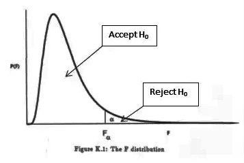
The type I error rate or significance level is the probability of rejecting the null hypothesis given that it is true. It is denoted by the Greek letter α (alpha) and is also called the alpha level. Often, the significance level is set to 0.05 (5%), implying that it is acceptable to have a 5% probability of incorrectly rejecting the null hypothesis.

Type II error

A type II error occurs when the null hypothesis is false, but erroneously fails to be rejected. It is failing to assert what is present, a miss. A type II error may be compared with a so-called false negative (where an actual ‘hit’ was disregarded by the test and seen as a ‘miss’) in a test checking for a single condition with a definitive result of true or false. A Type II error is committed when we fail to believe a true alternative hypothesis.

In terms of folk tales, an investigator may fail to see the wolf when it is present (“failing to raise an alarm”). Again, H0: no wolf.

The rate of the type II error is denoted by the Greek letter β (beta) and related to the power of a test (which equals 1−β).

Table of error types
Null hypothesis (H0) is
True False
Decision
about null
hypothesis (H0)
Don’t
reject
Correct inference

(true negative)

(probability = 1−α)

Type II error

(false negative)

(probability = β) 

Reject Type I error

(false positive)

(probability = α) 

Correct inference

(true positive)

(probability = 1−β)

Error Rate

A perfect test would have zero false positives and zero false negatives. However, statistical methods are probabilistic, and it cannot be known for certain whether statistical conclusions are correct. Whenever there is uncertainty, there is the possibility of making an error. Considering this nature of statistics science, all statistical hypothesis tests have a probability of making type I and type II errors.

  • The type I error rate or significance level is the probability of rejecting the null hypothesis given that it is true. It is denoted by the Greek letter α (alpha) and is also called the alpha level. Usually, the significance level is set to 0.05 (5%), implying that it is acceptable to have a 5% probability of incorrectly rejecting the true null hypothesis.
  • The rate of the type II error is denoted by the Greek letter β (beta) and related to the power of a test, which equals 1−β.

These two types of error rates are traded off against each other: for any given sample set, the effort to reduce one type of error generally results in increasing the other type of error.

The quality of hypothesis test

Error 2

The same idea can be expressed in terms of the rate of correct results and therefore used to minimize error rates and improve the quality of hypothesis test. To reduce the probability of committing a Type I error, making the alpha (p) value more stringent is quite simple and efficient. To decrease the probability of committing a Type II error, which is closely associated with analyses’ power, either increasing the test’s sample size or relaxing the alpha level could increase the analyses’ power. A test statistic is robust if the Type I error rate is controlled.

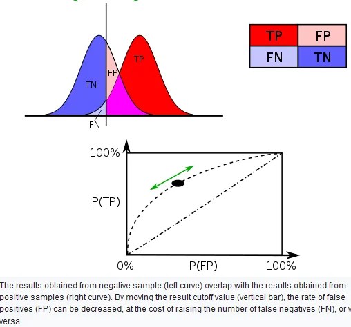
Varying different threshold (cut-off) value could also be used to make the test either more specific or more sensitive, which in turn elevates the test quality. For example, imagine a medical test, in which experimenter might measure the concentration of a certain protein in the blood sample. Experimenter could adjust the threshold (black vertical line in the figure) and people would be diagnosed as having diseases if any number is detected above this certain threshold. According to the image, changing the threshold would result in changes in false positives and false negatives, corresponding to movement on the curve.

Approximation

Too many results are only approximate; meaning they are similar but not equal to the actual result. An approximation can turn a complex calculation into a less complicated one.

For instance, the calculation of a Poisson distribution is more complicated than that of a binomial distribution. If both only differ slightly in their end result, it is permissible to approximate the Poisson distribution by a more simple-to-use binomial distribution. Prerequisite for such approximations is a sufficient sample size. In this example, at least 100 respondents are necessary in order to justify a sufficient proximity of the two distributions. An approximation based on too small a sample can lead to errors, for example, an accidental similarity of the two distributions.

The binomial distribution can be used to solve problems such as, “If a fair coin is flipped 100 times, what is the probability of getting 60 or more heads?” The probability of exactly x heads out of N

Flips is computed using the formula:

P(x)=[N!/(x!(N−x)!)]*πx(1−π)^N−x

where x

is the number of heads (60), N is the number of flips (100), and π

is the probability of a head (0.5). Therefore, to solve this problem, you compute the probability of 60 heads, then the probability of 61 heads, 62 heads, etc, and add up all these probabilities.

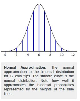
Abraham de Moivre, an 18th century statistician and consultant to gamblers, was often called upon to make these lengthy computations. de Moivre noted that when the number of events (coin flips) increased, the shape of the binomial distribution approached a very smooth curve. Therefore, de Moivre reasoned that if he could find a mathematical expression for this curve, he would be able to solve problems such as finding the probability of 60 or more heads out of 100 coin flips much more easily. This is exactly what he did, and the curve he discovered is now called the normal curve. The process of using this curve to estimate the shape of the binomial distribution is known as normal approximation.

Sixty two percent of 12th graders attend school in a particular urban school district. If a sample of 500 12th grade children are selected, find the probability that at least 290 are actually enrolled in school.

Part 1: Making the Calculations

Step 1: Find p,q, and n

  • The probability p is given in the question as 62%, or 0.62
  • To find q, subtract p from 1: 1 – 0.62 = 0.38
  • The sample size n is given in the question as 500

Step 2: Figure out if you can use the normal approximation to the binomial. If n * p and n * q are greater than 5, then you can use the approximation

n * p = 310 and n * q = 190.

These are both larger than 5, so you can use the normal approximation to the binomial for this question.

Step 3: Find the mean, μ by multiplying n and p

n * p = 310

(You actually figured that out in Step 2!).

Step 4: Multiply step 3 by q 

310 * 0.38 = 117.8.

Step 5: Take the square root of step 4 to get the standard deviation, σ

√(117.8)=10.85

Note: The formula for the standard deviation for a binomial is √(n*p*q)

Part 2: Using the Continuity Correction Factor

Step 6: Write the problem using correct notation. The question stated that we need to “find the probability that at least 290 are actually enrolled in school”. 

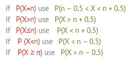
P(X ≥ 290)

Step 7: Rewrite the problem using the continuity correction factor

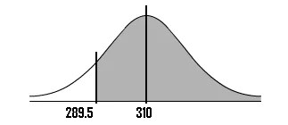
P (X ≥ 290-0.5) = P (X ≥ 289.5)

Step 8: Draw a diagram with the mean in the center. Shade the area that corresponds to the probability you are looking for. We’re looking for X ≥ 289.5, so:

Step 9: Find the z-score

You can find this by subtracting the mean (μ) from the probability you found in step 7, then dividing by the standard deviation (σ):

(289.5 – 310) / 10.85 = -1.89

Step 10: Look up the z-value in the z-table

The area for -1.89 is 0.4706.

Step 11: Add .5 to your answer in step 10 to find the total area pictured

0.4706 + 0.5 = 0.9706.

That’s it! The probability is .9706, or 97.06%.

Equity Market Meaning

An equity market is a platform that allows companies to raise capital via different investors. A company thus issues stock that investors or traders purchase in expectation of earning gains from future sales of said stock.

An equity market is a hub in which shares of companies are issued and traded. The market comes in the form of an exchange which facilitates the trade between buyers and sellers or over-the-counter (OTC) in which buyers and sellers find each other.

An equity market is a market in which shares of companies are issued and traded, either through exchanges or over-the-counter markets. Also known as the stock market, it is one of the most vital areas of a market economy. It gives companies access to capital to grow their business, and investors a piece of ownership in a company with the potential to realize gains in their investment based on the company’s future performance.

Equity Trading in the Stock Market

Trading in the equity market primarily entails the seller fixing a price and a buyer agreeing to pay that price to purchase the security, thus executing a sale. In a general context, the understanding of what is equity in the share market extends to all types of shares and securities traded that are also termed as stock. Equity and stock are thus used interchangeably for the purpose of trading.

Top Equity Exchanges

Some of the most well-known and largest equity markets are:

  • New York Stock Exchange (NYSE) – United States
  • Nasdaq (NASDAQ) – United States
  • Japan Exchange Group (JPX) – Japan
  • London Stock Exchange (LSE) – United Kingdom
  • Shanghai Stock Exchange (SSE) – China
  • Hong Kong Stock Exchange (HKEX) – Hong Kong
  • Euronext – European Union
  • Toronto Stock Exchange – Canada
  • Bombay Stock Exchange – India

Types of Equity Market

Equity markets comprise structured trading and investment and can be defined into two types of platforms, i.e., primary and secondary markets.

Primary market

Each company plans to offer its shares for public trading must start with Initial Public Offering or IPO. In this process, the company offers a part of its total equity to the public for raising capital initially. Once the IPO is complete, the stocks so offered are listed on the stock exchange for further trading.

The entire process of introducing the IPO by a company takes place in the primary market. In other words, this market comprises only the IPO introduction and investment.

Secondary market

Once the shares have already been listed on either of the exchanges, further trading for them is held in the secondary market. Here, the initial investors get an opportunity to exit their investments via stock sale in this live equity market. These stocks can comprise shares, along with other types of securities that can include convertible bonds, corporate bonds, etc.

error: Content is protected !!