Statistical Errors and Approximation

Statistical Errors and Approximation are important concepts in Business Statistics-I because statistical results may differ from the actual or true values due to various reasons. Statistical errors arise during data collection, sampling, measurement, processing, calculation, or interpretation. Approximation means expressing an exact value in a simpler form by rounding or estimating it. Understanding these concepts helps maintain accuracy, reliability, and consistency in statistical calculations and investigations.

1. Statistical Error

Statistical Error is the difference between the true value of a population characteristic and the value obtained through statistical observation or calculation. Errors may occur because of sampling, measurement, recording, processing, or other factors. Statistical error does not necessarily mean that an investigator has made a mistake; some errors are unavoidable when studying a sample rather than the complete population.

Example: If the actual average monthly income of a population is ₹35,000 but the calculated sample average is ₹34,500, the difference of ₹500 represents statistical error.

2. Sampling Error

Sampling Error occurs because a sample rather than the entire population is studied. Even when sampling is carried out correctly, the characteristics of a sample may differ from those of the population. The size of sampling error depends on factors such as sample size, sampling method, and population variability. A larger and properly selected sample generally reduces sampling error.

Example: The actual average expenditure of all customers is ₹8,000, while a selected sample of customers shows an average of ₹7,700. The difference represents sampling error.

3. Non-Sampling Error

Non-Sampling Error arises from factors other than sampling and can occur in both census and sample investigations. Common causes include incorrect responses, poor questionnaire design, missing information, interviewer bias, recording mistakes, and data-processing errors. These errors can sometimes be more serious than sampling errors because increasing the sample size does not necessarily eliminate them.

Example: If respondents incorrectly report their monthly income because they misunderstand the question, the resulting incorrect information represents a non-sampling error.

4. Measurement Error

Measurement Error occurs when the value recorded during an investigation differs from the actual value of the variable being measured. It may result from defective instruments, inaccurate procedures, unclear definitions, or misunderstanding by respondents. Proper measurement standards and reliable instruments can help minimize such errors.

Example: If the actual weight of a product is 10 kilograms but an improperly calibrated weighing machine records it as 9.8 kilograms, the difference of 0.2 kilograms represents a measurement error.

5. Processing and Calculation Error

Processing and Calculation Errors occur during editing, coding, classification, tabulation, data entry, or mathematical calculations. Even accurate data can produce incorrect results if mistakes are made while processing them. Such errors may include incorrect addition, duplication of observations, wrong coding, or entering figures incorrectly. Careful checking and verification are necessary to reduce these errors.

Example: If the sales figures ₹20,000, ₹30,000, and ₹40,000 are incorrectly added as ₹80,000 instead of ₹90,000, the resulting figure contains a calculation error.

6. Approximation

Approximation means representing an exact numerical value by a nearby simpler value. It is commonly used when exact values contain many decimal places or when a simpler figure is sufficient for practical purposes. Approximation makes statistical calculations and presentation easier, but it introduces a small difference from the exact value.

Example: If the exact average sales value is ₹25,678.45, it may be approximated to ₹25,678 or ₹25,700 depending on the required level of accuracy. The choice should be appropriate to the purpose.

7. Rounding Off

Rounding Off is a common method of approximation in which numbers are reduced to a specified number of decimal places or significant digits. If the next digit is 5 or more, the preceding digit is generally increased by one; if it is less than 5, the preceding digit remains unchanged. Consistent rounding improves clarity and presentation.

Example: 48.736 rounded to two decimal places becomes 48.74, while 48.732 becomes 48.73. Rounding should be performed carefully to avoid unnecessary errors.

8. Absolute and Relative Error

Absolute Error is the numerical difference between the true value and the observed or approximate value. Relative Error expresses this difference in relation to the true value and is often presented as a percentage. These measures help determine the magnitude and significance of an error.

Example: If the true value is 500 and the observed value is 490, the absolute error is 10. The relative error is 10 ÷ 500 × 100 = 2%. Thus, relative error provides a useful measure of accuracy.

A type I error (or error of the first kind) is the incorrect rejection of a true null hypothesis. Usually, a type I error leads one to conclude that a supposed effect or relationship exists when in fact it doesn’t. Examples of type I errors include a test that shows a patient to have a disease when in fact the patient does not have the disease, a fire alarm going on indicating a fire when in fact there is no fire, or an experiment indicating that a medical treatment should cure a disease when in fact it does not.

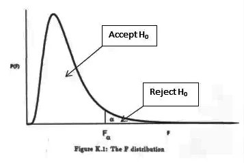
A type II error (or error of the second kind) is the failure to reject a false null hypothesis. Examples of type II errors would be a blood test failing to detect the disease it was designed to detect, in a patient who really has the disease; a fire breaking out and the fire alarm does not ring; or a clinical trial of a medical treatment failing to show that the treatment works when really it does.

When comparing two means, concluding the means were different when in reality they were not different would be a Type I error; concluding the means were not different when in reality they were different would be a Type II error. Various extensions have been suggested as “Type III errors”, though none have wide use.

All statistical hypothesis tests have a probability of making type I and type II errors. For example, all blood tests for a disease will falsely detect the disease in some proportion of people who don’t have it, and will fail to detect the disease in some proportion of people who do have it. A test’s probability of making a type I error is denoted by α. A test’s probability of making a type II error is denoted by β. These error rates are traded off against each other: for any given sample set, the effort to reduce one type of error generally results in increasing the other type of error. For a given test, the only way to reduce both error rates is to increase the sample size, and this may not be feasible.

Type I error

A type I error occurs when the null hypothesis (H0) is true, but is rejected. It is asserting something that is absent, a false hit. A type I error may be likened to a so-called false positive (a result that indicates that a given condition is present when it actually is not present).

In terms of folk tales, an investigator may see the wolf when there is none (“raising a false alarm”). Where the null hypothesis, H0, is: no wolf.

The type I error rate or significance level is the probability of rejecting the null hypothesis given that it is true. It is denoted by the Greek letter α (alpha) and is also called the alpha level. Often, the significance level is set to 0.05 (5%), implying that it is acceptable to have a 5% probability of incorrectly rejecting the null hypothesis.

Type II error

A type II error occurs when the null hypothesis is false, but erroneously fails to be rejected. It is failing to assert what is present, a miss. A type II error may be compared with a so-called false negative (where an actual ‘hit’ was disregarded by the test and seen as a ‘miss’) in a test checking for a single condition with a definitive result of true or false. A Type II error is committed when we fail to believe a true alternative hypothesis.

In terms of folk tales, an investigator may fail to see the wolf when it is present (“failing to raise an alarm”). Again, H0: no wolf.

The rate of the type II error is denoted by the Greek letter β (beta) and related to the power of a test (which equals 1−β).

Table of error types		Null hypothesis (H0) is
		True	False
Decision about null hypothesis (H0)	Don’t reject	Correct inference (true negative) (probability = 1−α)	Type II error (false negative) (probability = β)
	Reject	Type I error (false positive) (probability = α)	Correct inference (true positive) (probability = 1−β)

Error Rate

A perfect test would have zero false positives and zero false negatives. However, statistical methods are probabilistic, and it cannot be known for certain whether statistical conclusions are correct. Whenever there is uncertainty, there is the possibility of making an error. Considering this nature of statistics science, all statistical hypothesis tests have a probability of making type I and type II errors.

• The type I error rate or significance level is the probability of rejecting the null hypothesis given that it is true. It is denoted by the Greek letter α (alpha) and is also called the alpha level. Usually, the significance level is set to 0.05 (5%), implying that it is acceptable to have a 5% probability of incorrectly rejecting the true null hypothesis.
• The rate of the type II error is denoted by the Greek letter β (beta) and related to the power of a test, which equals 1−β.

These two types of error rates are traded off against each other: for any given sample set, the effort to reduce one type of error generally results in increasing the other type of error.

The quality of hypothesis test

Error 2

The same idea can be expressed in terms of the rate of correct results and therefore used to minimize error rates and improve the quality of hypothesis test. To reduce the probability of committing a Type I error, making the alpha (p) value more stringent is quite simple and efficient. To decrease the probability of committing a Type II error, which is closely associated with analyses’ power, either increasing the test’s sample size or relaxing the alpha level could increase the analyses’ power. A test statistic is robust if the Type I error rate is controlled.

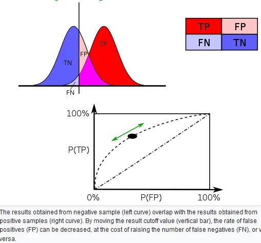
Varying different threshold (cut-off) value could also be used to make the test either more specific or more sensitive, which in turn elevates the test quality. For example, imagine a medical test, in which experimenter might measure the concentration of a certain protein in the blood sample. Experimenter could adjust the threshold (black vertical line in the figure) and people would be diagnosed as having diseases if any number is detected above this certain threshold. According to the image, changing the threshold would result in changes in false positives and false negatives, corresponding to movement on the curve.

Approximation

Too many results are only approximate; meaning they are similar but not equal to the actual result. An approximation can turn a complex calculation into a less complicated one.

For instance, the calculation of a Poisson distribution is more complicated than that of a binomial distribution. If both only differ slightly in their end result, it is permissible to approximate the Poisson distribution by a more simple-to-use binomial distribution. Prerequisite for such approximations is a sufficient sample size. In this example, at least 100 respondents are necessary in order to justify a sufficient proximity of the two distributions. An approximation based on too small a sample can lead to errors, for example, an accidental similarity of the two distributions.

The binomial distribution can be used to solve problems such as, “If a fair coin is flipped 100 times, what is the probability of getting 60 or more heads?” The probability of exactly x heads out of N

Flips is computed using the formula:

P(x)=[N!/(x!(N−x)!)]*πx(1−π)^N−x

where x

is the number of heads (60), N is the number of flips (100), and π

is the probability of a head (0.5). Therefore, to solve this problem, you compute the probability of 60 heads, then the probability of 61 heads, 62 heads, etc, and add up all these probabilities.

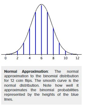
Abraham de Moivre, an 18th century statistician and consultant to gamblers, was often called upon to make these lengthy computations. de Moivre noted that when the number of events (coin flips) increased, the shape of the binomial distribution approached a very smooth curve. Therefore, de Moivre reasoned that if he could find a mathematical expression for this curve, he would be able to solve problems such as finding the probability of 60 or more heads out of 100 coin flips much more easily. This is exactly what he did, and the curve he discovered is now called the normal curve. The process of using this curve to estimate the shape of the binomial distribution is known as normal approximation.

Sixty two percent of 12th graders attend school in a particular urban school district. If a sample of 500 12th grade children are selected, find the probability that at least 290 are actually enrolled in school.

Part 1: Making the Calculations

Step 1: Find p,q, and n

• The probability p is given in the question as 62%, or 0.62
• To find q, subtract p from 1: 1 – 0.62 = 0.38
• The sample size n is given in the question as 500

Step 2: Figure out if you can use the normal approximation to the binomial. If n * p and n * q are greater than 5, then you can use the approximation

n * p = 310 and n * q = 190.

These are both larger than 5, so you can use the normal approximation to the binomial for this question.

Step 3: Find the mean, μ by multiplying n and p

n * p = 310

(You actually figured that out in Step 2!).

Step 4: Multiply step 3 by q 

310 * 0.38 = 117.8.

Step 5: Take the square root of step 4 to get the standard deviation, σ

√(117.8)=10.85

Note: The formula for the standard deviation for a binomial is √(n*p*q)

Part 2: Using the Continuity Correction Factor

Step 6: Write the problem using correct notation. The question stated that we need to “find the probability that at least 290 are actually enrolled in school”. 

P(X ≥ 290)

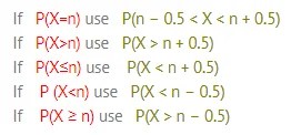
Step 7: Rewrite the problem using the continuity correction factor

P (X ≥ 290-0.5) = P (X ≥ 289.5)

Step 8: Draw a diagram with the mean in the center. Shade the area that corresponds to the probability you are looking for. We’re looking for X ≥ 289.5, so:

Step 9: Find the z-score

You can find this by subtracting the mean (μ) from the probability you found in step 7, then dividing by the standard deviation (σ):

(289.5 – 310) / 10.85 = -1.89

Step 10: Look up the z-value in the z-table

The area for -1.89 is 0.4706.

Step 11: Add .5 to your answer in step 10 to find the total area pictured

0.4706 + 0.5 = 0.9706.

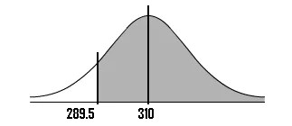
That’s it! The probability is .9706, or 97.06%.