Determinants of the Value of Bonds

Bonds are fixed-income securities that represent a loan from an investor to a borrower, typically a corporation or government. When purchasing a bond, the investor lends money in exchange for periodic interest payments and the return of the bond’s face value at maturity. Bonds are used to finance various projects and operations, providing a predictable income stream for investors.

Valuation of Bonds

The method for valuation of bonds involves three steps as follows:

Step 1: Estimate the expected cash flows

Step 2: Determine the appropriate interest rate that should be used to discount the cash flows.

& Step 3: Calculate the present value of the expected cash flows (step-1) using appropriate interest rate (step- 2) i.e. discounting the expected cash flows

Step 1: Estimating cash flows

Cash flow is the cash that is estimated to be received in future from investment in a bond. There are only two types of cash flows that can be received from investment in bonds i.e. coupon payments and principal payment at maturity.

The usual cash flow cycle of the bond is coupon payments are received at regular intervals as per the bond agreement, and final coupon plus principle payment is received at the maturity. There are some instances when bonds don’t follow these regular patterns. Unusual patterns maybe a result of the different type of bond such as zero-coupon bonds, in which there are no coupon payments. Considering such factors, it is important for an analyst to estimate accurate cash flow for the purpose of bond valuation.

Step 2: Determine the appropriate interest rate to discount the cash flows

Once the cash flow for the bond is estimated, the next step is to determine the appropriate interest rate to discount cash flows. The minimum interest rate that an investor should require is the interest available in the marketplace for default-free cash flow. Default-free cash flows are cash flows from debt security which are completely safe and has zero chances default. Such securities are usually issued by the central bank of a country, for example, in the USA it is bonds by U.S. Treasury Security.

Consider a situation where an investor wants to invest in bonds. If he is considering to invest corporate bonds, he is expecting to earn higher return from these corporate bonds compared to rate of returns of U.S. Treasury Security bonds. This is because chances are that a corporate bond might default, whereas the U.S. Security Treasury bond is never going to default. As he is taking a higher risk by investing in corporate bonds, he expects a higher return.

One may use single interest rate or multiple interest rates for valuation.

Step 3: Discounting the expected cash flows

Now that we already have values of expected future cash flows and interest rate used to discount the cash flow, it is time to find the present value of cash flows. Present Value of a cash flow is the amount of money that must be invested today to generate a specific future value. The present value of a cash flow is more commonly known as discounted value.

The present value of a cash flow depends on two determinants:

  • When a cash flow will be received i.e. timing of a cash flow &;
  • The required interest rate, more widely known as Discount Rate (rate as per Step-2)

First, we calculate the present value of each expected cash flow. Then we add all the individual present values and the resultant sum is the value of the bond.

The formula to find the present value of one cash flow is:

Present value formula for Bond Valuation

Present Value n = Expected cash flow in the period n/ (1+i) n

Here,

i = rate of return/discount rate on bond
n = expected time to receive the cash flow

By this formula, we will get the present value of each individual cash flow t years from now. The next step is to add all individual cash flows.

Bond Value = Present Value 1 + Present Value 2 + ……. + Present Value n

Research, Introduction, Meaning, Definition, Objective, Purpose, Types, Importance and Challenges

Research is a systematic and organized process of collecting, analyzing, and interpreting information to increase understanding of a topic or issue. It aims to discover new facts, verify existing knowledge, or solve specific problems through careful investigation. Research can be theoretical or applied, and it involves forming hypotheses, gathering data, and drawing conclusions. It is essential in academic, scientific, and business fields to make informed decisions and improve practices. A well-conducted research study follows a structured methodology to ensure reliability and validity. Overall, research is a tool for expanding knowledge and contributing to the development of society and industries.

Definition of Research

  • Clifford Woody

Research is a careful inquiry or examination to discover new facts or verify old ones.

  • Creswell

Research is a process of steps used to collect and analyze information to increase our understanding of a topic.

  • Redman and Mory

Research is a systematized effort to gain new knowledge.

  • Kerlinger

Research is a systematic, controlled, empirical, and critical investigation of hypothetical propositions.

  • Lundberg

Research is a systematic activity directed towards the discovery and development of an organized body of knowledge.

Objective of Research

  • To Gain Familiarity with a Phenomenon

One major objective of research is to explore and understand a phenomenon or concept more clearly. This is often done through exploratory research, especially when little prior knowledge exists. It helps researchers gain insights into new topics, identify trends, and lay the groundwork for future studies. By becoming familiar with unfamiliar issues, researchers can form better hypotheses and research questions. This foundational understanding is critical for developing more in-depth research and creating meaningful contributions to academic and professional fields.

  • To Describe a Phenomenon Accurately

Descriptive research aims to systematically and precisely describe the characteristics of a subject, event, or population. Whether it’s human behavior, market trends, or institutional processes, this type of research collects detailed information to create an accurate picture. The objective is not to determine cause-and-effect but to define “what is” in a clear and factual manner. Such descriptions help researchers, practitioners, and policymakers understand the current state of affairs and serve as a reference point for comparing future changes.

  • To Establish Cause-and-Effect Relationships

Causal or explanatory research seeks to identify and analyze relationships between variables, often using experiments or observational studies. The objective is to determine how and why certain phenomena occur. For instance, a business might study the impact of advertising on sales. Establishing cause-and-effect allows researchers to predict outcomes and design effective interventions. This type of research is essential in fields like science, economics, and medicine, where understanding the effects of one factor on another can lead to critical discoveries and solutions.

  • To Test Hypotheses

Another key objective of research is hypothesis testing, where assumptions or predictions made before a study are examined for accuracy. Researchers design experiments or surveys to gather data that supports or refutes their hypotheses. The goal is to provide empirical evidence for or against theoretical statements. This process sharpens theories, confirms findings, and promotes scientific accuracy. Testing hypotheses is particularly important in quantitative research, as it relies on statistical techniques to validate conclusions and ensure objectivity.

  • To Develop New Theories and Concepts

Research often leads to the creation or refinement of theories and models that explain how the world works. The objective here is to go beyond existing knowledge and offer new perspectives or conceptual frameworks. Through in-depth analysis, researchers can challenge outdated views and propose innovative explanations. These new theories guide future research, inform policy, and influence practice across disciplines. In academic fields, theoretical research forms the basis for scholarly progress and intellectual advancement.

  • To Find Solutions to Practical Problems

Applied research is conducted with the specific objective of solving real-world problems. Whether it’s improving product design, enhancing public health, or increasing workplace efficiency, the goal is to apply scientific methods to practical challenges. This kind of research is widely used in industries, education, and government. It not only addresses current issues but also anticipates future needs. By developing effective strategies and solutions, applied research makes a direct contribution to societal well-being and economic development.

  • To Predict Future Trends

Research aims to forecast what may happen in the future based on current and past data. Predictive research uses statistical tools and modeling techniques to identify patterns and trends that inform future outcomes. For example, businesses use market research to predict consumer behavior, and climate scientists use data to forecast environmental changes. These predictions guide planning and strategic decisions. Accurate forecasting is essential for minimizing risk, improving preparedness, and making proactive decisions in dynamic environments.

  • To Enhance Understanding and Clarify Doubts

Research helps deepen our understanding of complex topics and clarifies uncertainties that may exist in previous studies or beliefs. By investigating issues from multiple angles, using various methods, and verifying results, research ensures greater clarity and accuracy. This objective is crucial in academia and science, where incomplete or conflicting information often leads to confusion. Ongoing research contributes to refinement, resolution of debates, and filling knowledge gaps, ensuring a more complete and reliable understanding of any subject.

Purpose of Research

  • Discovery of New Knowledge

One of the primary purposes of research is to discover new facts, ideas, and knowledge. Research helps in expanding the existing pool of information by exploring unknown areas and generating fresh insights. Through systematic investigation, researchers identify new relationships, concepts, and principles that were previously unexplored. This contributes to the growth of various disciplines such as science, management, economics, and social sciences. Discovery-oriented research lays the foundation for innovation, development, and further academic inquiry in different fields of study.

  • Verification of Existing Knowledge

Research is conducted to test and verify the validity of existing theories, laws, and concepts. Many ideas accepted over time require re-examination due to changing conditions, new evidence, or technological advancements. Research helps confirm whether earlier findings are still relevant and accurate. This process strengthens the reliability of knowledge by removing errors, misconceptions, and outdated assumptions. Verification through research ensures that decisions, policies, and practices are based on dependable and scientifically tested information.

  • Solution to Practical Problems

Another important purpose of research is to provide solutions to real-life problems faced by individuals, organizations, industries, and society. Applied research focuses on identifying causes of problems and suggesting effective remedies. In business, research helps solve issues related to production, marketing, finance, and human resources. In social sciences, it addresses problems like poverty, unemployment, and health. Thus, research acts as a tool for problem-solving and practical decision-making.

  • Development of Theories and Concepts

Research helps in developing new theories, models, and conceptual frameworks. By analyzing data and observing patterns, researchers formulate generalizations and principles that explain phenomena. These theories provide a systematic understanding of relationships among variables and guide future research. Theory-building research enhances academic depth and strengthens subject foundations. It also helps practitioners apply theoretical knowledge in practical situations, thereby bridging the gap between theory and practice in various disciplines.

  • Prediction and Forecasting

Research plays a significant role in predicting future trends and outcomes. By studying past and present data, researchers can forecast changes in markets, consumer behavior, population growth, and economic conditions. Such predictions help organizations and governments plan for the future and reduce uncertainty. Forecasting through research supports strategic planning, risk management, and policy formulation. Accurate predictions enable better preparedness for challenges and opportunities that may arise in the future.

  • Improvement in Decision Making

One of the key purposes of research is to support sound and rational decision-making. Research provides relevant, accurate, and timely information required for making informed choices. In business and management, research reduces guesswork and reliance on intuition. Decisions related to investment, product development, and policy implementation become more effective when backed by research findings. Thus, research improves the quality of decisions and enhances efficiency and effectiveness in achieving objectives.

  • Advancement of Social and Economic Development

Research contributes significantly to social and economic progress. It helps identify social issues, evaluate government programs, and suggest improvements in public policies. Economic research aids in understanding growth patterns, inflation, employment, and income distribution. Through research, innovative solutions are developed to improve living standards and promote sustainable development. Hence, research supports national development by providing a scientific basis for planning, reforms, and welfare initiatives.

  • Enhancement of Knowledge and Learning

Research promotes intellectual growth and continuous learning. It develops analytical thinking, creativity, and problem-solving abilities among researchers and students. Through research, individuals gain deeper understanding of subjects and develop a scientific attitude. It encourages questioning, exploration, and logical reasoning. This purpose is especially important in education, where research-based learning improves academic quality and contributes to personal and professional development.

Types of Research

1. Basic Research

Basic research, also known as pure or fundamental research, is conducted to expand existing knowledge without focusing on immediate practical application. Its main objective is to develop theories, principles, and generalizations. This type of research helps in understanding fundamental aspects of a subject and provides a foundation for applied research. Although it may not offer direct solutions, basic research is essential for long-term academic growth and scientific advancement.

2. Applied Research

Applied research is undertaken to solve specific, practical problems faced by individuals, organizations, or society. It focuses on applying theoretical knowledge to real-life situations. This type of research is common in fields like business, management, medicine, and engineering. The findings of applied research are directly useful for decision-making and problem-solving. It helps improve products, processes, and services by providing workable solutions.

3. Descriptive Research

Descriptive research aims to describe the characteristics of a population, situation, or phenomenon accurately. It does not control variables but observes and reports conditions as they exist. Surveys, questionnaires, and observational methods are commonly used. This type of research helps in understanding “what is happening” rather than “why it happens.” Descriptive research is widely used in social sciences, marketing, and business studies.

4. Analytical Research

Analytical research involves the use of existing data to analyze and evaluate relationships among variables. The researcher critically examines facts and information to draw conclusions. Unlike descriptive research, analytical research focuses on “why” and “how” aspects. It requires logical reasoning and statistical tools. This type of research is useful in policy analysis, financial studies, and economic research to understand cause-and-effect relationships.

5. Exploratory Research

Exploratory research is conducted when a problem is not clearly defined or when little information is available. Its purpose is to gain initial insights and understanding of the problem. Methods such as interviews, focus groups, and literature reviews are commonly used. Exploratory research helps in formulating hypotheses and identifying variables for further study. It provides direction for more detailed and structured research.

6. Qualitative Research

Qualitative research focuses on understanding human behavior, opinions, and experiences in a non-numerical form. It uses methods like interviews, case studies, and observations. This type of research emphasizes depth rather than quantity of data. Qualitative research helps in exploring attitudes, motivations, and perceptions. It is widely used in social sciences, psychology, and management to gain detailed insights.

7. Quantitative Research

Quantitative research deals with numerical data and statistical analysis. It aims to quantify variables and examine relationships using structured tools like surveys and experiments. This type of research provides measurable and objective results. Quantitative research is useful for testing hypotheses and making generalizations. It is commonly used in business, economics, and scientific studies where precision and accuracy are required.

8. Conceptual and Empirical Research

Conceptual research is based on abstract ideas, theories, and concepts. It involves logical reasoning and theoretical analysis without relying on observation. Empirical research, on the other hand, is based on actual observations and experiments. It relies on data collection and evidence. Both types are important, as conceptual research builds theories, while empirical research tests and validates them in real-world conditions.

Importance of Research

  • Expansion of Knowledge

Research plays a vital role in expanding human knowledge. It helps us understand concepts, theories, and facts in a deeper and more meaningful way. Through systematic investigation, research uncovers hidden truths and broadens the scope of what is already known. This continuous process of discovery is essential in education, science, and innovation. Without research, the development of new ideas, improvements in technology, and advancements in various fields would come to a standstill.

  • Problem Solving

One of the main purposes of research is to find solutions to problems. In both academic and practical settings, research helps identify the root causes of issues and suggests possible remedies. Whether it’s a social, economic, scientific, or business problem, research provides the tools and frameworks to analyze the situation effectively. It allows decision-makers to make evidence-based choices and implement strategies that are backed by data and analysis, leading to more successful outcomes.

  • Informed Decision Making

Research enables individuals, organizations, and governments to make informed decisions. By analyzing data and studying trends, research provides a factual basis for choosing between alternatives. In business, it helps managers decide on product development, marketing strategies, and investment plans. In public policy, it helps lawmakers craft laws that address real needs. This reduces the risk of failure and ensures that decisions are effective, efficient, and aligned with actual conditions and demands.

  • Economic Development

Research is essential for economic growth and development. It leads to the creation of new products, services, and technologies, which drive industry and generate employment. By improving productivity, reducing costs, and increasing competitiveness, research directly contributes to the success of businesses and national economies. Additionally, research in areas like agriculture, health, and education ensures sustainable development by solving real-world problems and improving the quality of life for individuals and communities.

  • Improvement in Education

Research strengthens the education system by improving teaching methods, learning outcomes, and academic content. It helps educators understand student needs, evaluate curricula, and adopt innovative practices. Research also enables students and teachers to stay updated with the latest knowledge in their field, promoting lifelong learning. Educational research contributes to the development of better textbooks, e-learning tools, and inclusive teaching strategies that cater to diverse learning styles and backgrounds.

  • Policy Formulation

Government and institutional policies must be based on reliable data and analysis, which research provides. Whether in health, education, environment, or public safety, research ensures that policies are relevant, effective, and future-ready. It helps policymakers assess the potential impact of laws and regulations, avoiding guesswork and promoting social welfare. Evidence-based policies are more likely to gain public support and achieve their goals, ultimately benefiting the economy and society as a whole.

  • Innovation and Technology Advancement

Innovation thrives on research. From developing new medical treatments to designing smarter devices, research is the foundation of technological progress. Scientists and engineers rely on research to explore possibilities, test ideas, and turn concepts into real-world applications. Research also encourages creativity and collaboration across disciplines, pushing the boundaries of what’s possible. As technology rapidly evolves, research ensures that innovation continues to meet the needs of people and adapt to changing environments.

  • Social and Cultural Understanding

Research deepens our understanding of social and cultural dynamics. It helps explore human behavior, beliefs, traditions, and societal changes. Through research in fields like sociology, anthropology, and psychology, we gain insights into communities and cultures, fostering tolerance and mutual respect. This understanding is crucial in a globalized world where collaboration and coexistence are key. It also helps in addressing social issues like poverty, gender inequality, and discrimination with informed, data-backed strategies.

Challenges in Research

  • Problem Identification and Definition

One of the major challenges in research is identifying and clearly defining the research problem. An unclear or poorly framed problem leads to confusion and ineffective results. Researchers often face difficulty in narrowing down a broad topic into a specific and researchable problem. Lack of clarity affects objectives, hypothesis formulation, and methodology. Proper understanding of the problem is essential, as the entire research process depends on accurate problem identification and precise definition.

  • Availability of Reliable Data

Availability of accurate and reliable data is a significant challenge in research. Researchers may face incomplete, outdated, or inconsistent data sources. In some cases, data may not be accessible due to confidentiality or restrictions. Primary data collection can be costly and time-consuming, while secondary data may lack relevance. Poor quality data directly affects the validity and reliability of research findings, making conclusions less dependable.

  • Time Constraints

Time limitation is a common challenge faced by researchers, especially students and professionals. Research involves multiple stages such as literature review, data collection, analysis, and reporting, each requiring adequate time. Due to academic deadlines or organizational pressure, researchers may rush through processes, leading to errors and superficial analysis. Insufficient time affects depth, accuracy, and overall quality of research work.

  • Financial Constraints

Lack of adequate funds poses a major challenge in conducting research. Expenses related to data collection, fieldwork, surveys, software, and expert consultation can be high. Limited financial resources restrict sample size, research tools, and scope of the study. Due to budget constraints, researchers may compromise on quality and methodology, which negatively impacts the reliability and effectiveness of research outcomes.

  • Selection of Appropriate Research Methodology

Choosing the correct research methodology is often challenging. Researchers may struggle to select suitable research design, sampling techniques, and data collection methods. Incorrect methodology leads to biased results and invalid conclusions. Lack of experience or guidance further complicates this challenge. Proper alignment between research objectives and methodology is crucial to ensure meaningful and accurate findings.

  • Researcher Bias and Subjectivity

Researcher bias is a serious challenge that affects objectivity. Personal beliefs, assumptions, and expectations may influence data collection, interpretation, and conclusions. Bias can occur intentionally or unintentionally, leading to distorted results. Maintaining neutrality and using standardized tools is essential. Overcoming bias requires awareness, ethical conduct, and adherence to scientific principles throughout the research process.

  • Ethical Issues in Research

Ethical challenges are common in research involving human subjects. Issues such as informed consent, privacy, confidentiality, and data misuse must be carefully handled. Researchers may face difficulty in balancing research objectives with ethical responsibilities. Failure to follow ethical standards can lead to legal consequences and loss of credibility. Ethical compliance is essential for responsible and trustworthy research.

  • Data Analysis and Interpretation

Analyzing and interpreting data accurately is a complex challenge in research. Researchers may lack technical knowledge of statistical tools and software. Misinterpretation of data can lead to incorrect conclusions. Large volumes of data increase complexity and chances of error. Proper training, use of appropriate analytical techniques, and careful interpretation are necessary to ensure valid and meaningful research results.

Sampling and Sampling Distribution

Sample design is the framework, or road map, that serves as the basis for the selection of a survey sample and affects many other important aspects of a survey as well. In a broad context, survey researchers are interested in obtaining some type of information through a survey for some population, or universe, of interest. One must define a sampling frame that represents the population of interest, from which a sample is to be drawn. The sampling frame may be identical to the population, or it may be only part of it and is therefore subject to some under coverage, or it may have an indirect relationship to the population.

Sampling is the process of selecting a subset of individuals, items, or observations from a larger population to analyze and draw conclusions about the entire group. It is essential in statistics when studying the entire population is impractical, time-consuming, or costly. Sampling can be done using various methods, such as random, stratified, cluster, or systematic sampling. The main objectives of sampling are to ensure representativeness, reduce costs, and provide timely insights. Proper sampling techniques enhance the reliability and validity of statistical analysis and decision-making processes.

Steps in Sample Design

While developing a sampling design, the researcher must pay attention to the following points:

  • Type of Universe:

The first step in developing any sample design is to clearly define the set of objects, technically called the Universe, to be studied. The universe can be finite or infinite. In finite universe the number of items is certain, but in case of an infinite universe the number of items is infinite, i.e., we cannot have any idea about the total number of items. The population of a city, the number of workers in a factory and the like are examples of finite universes, whereas the number of stars in the sky, listeners of a specific radio programme, throwing of a dice etc. are examples of infinite universes.

  • Sampling unit:

A decision has to be taken concerning a sampling unit before selecting sample. Sampling unit may be a geographical one such as state, district, village, etc., or a construction unit such as house, flat, etc., or it may be a social unit such as family, club, school, etc., or it may be an individual. The researcher will have to decide one or more of such units that he has to select for his study.

  • Source list:

It is also known as ‘sampling frame’ from which sample is to be drawn. It contains the names of all items of a universe (in case of finite universe only). If source list is not available, researcher has to prepare it. Such a list should be comprehensive, correct, reliable and appropriate. It is extremely important for the source list to be as representative of the population as possible.

  • Size of Sample:

This refers to the number of items to be selected from the universe to constitute a sample. This a major problem before a researcher. The size of sample should neither be excessively large, nor too small. It should be optimum. An optimum sample is one which fulfills the requirements of efficiency, representativeness, reliability and flexibility. While deciding the size of sample, researcher must determine the desired precision as also an acceptable confidence level for the estimate. The size of population variance needs to be considered as in case of larger variance usually a bigger sample is needed. The size of population must be kept in view for this also limits the sample size. The parameters of interest in a research study must be kept in view, while deciding the size of the sample. Costs too dictate the size of sample that we can draw. As such, budgetary constraint must invariably be taken into consideration when we decide the sample size.

  • Parameters of interest:

In determining the sample design, one must consider the question of the specific population parameters which are of interest. For instance, we may be interested in estimating the proportion of persons with some characteristic in the population, or we may be interested in knowing some average or the other measure concerning the population. There may also be important sub-groups in the population about whom we would like to make estimates. All this has a strong impact upon the sample design we would accept.

  • Budgetary constraint:

Cost considerations, from practical point of view, have a major impact upon decisions relating to not only the size of the sample but also to the type of sample. This fact can even lead to the use of a non-probability sample.

  • Sampling procedure:

Finally, the researcher must decide the type of sample he will use i.e., he must decide about the technique to be used in selecting the items for the sample. In fact, this technique or procedure stands for the sample design itself. There are several sample designs (explained in the pages that follow) out of which the researcher must choose one for his study. Obviously, he must select that design which, for a given sample size and for a given cost, has a smaller sampling error.

Types of Samples

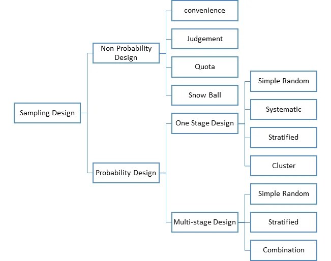
  • Probability Sampling (Representative samples)

Probability samples are selected in such a way as to be representative of the population. They provide the most valid or credible results because they reflect the characteristics of the population from which they are selected (e.g., residents of a particular community, students at an elementary school, etc.). There are two types of probability samples: random and stratified.

  • Random Sample

The term random has a very precise meaning. Each individual in the population of interest has an equal likelihood of selection. This is a very strict meaning you can’t just collect responses on the street and have a random sample.

The assumption of an equal chance of selection means that sources such as a telephone book or voter registration lists are not adequate for providing a random sample of a community. In both these cases there will be a number of residents whose names are not listed. Telephone surveys get around this problem by random-digit dialling but that assumes that everyone in the population has a telephone. The key to random selection is that there is no bias involved in the selection of the sample. Any variation between the sample characteristics and the population characteristics is only a matter of chance.

  • Stratified Sample

A stratified sample is a mini-reproduction of the population. Before sampling, the population is divided into characteristics of importance for the research. For example, by gender, social class, education level, religion, etc. Then the population is randomly sampled within each category or stratum. If 38% of the population is college-educated, then 38% of the sample is randomly selected from the college-educated population.

Stratified samples are as good as or better than random samples, but they require fairly detailed advance knowledge of the population characteristics, and therefore are more difficult to construct.

  • Non-probability Samples (Non-representative samples)

As they are not truly representative, non-probability samples are less desirable than probability samples. However, a researcher may not be able to obtain a random or stratified sample, or it may be too expensive. A researcher may not care about generalizing to a larger population. The validity of non-probability samples can be increased by trying to approximate random selection, and by eliminating as many sources of bias as possible.

  • Quota Sample

The defining characteristic of a quota sample is that the researcher deliberately sets the proportions of levels or strata within the sample. This is generally done to insure the inclusion of a particular segment of the population. The proportions may or may not differ dramatically from the actual proportion in the population. The researcher sets a quota, independent of population characteristics.

Example: A researcher is interested in the attitudes of members of different religions towards the death penalty. In Iowa a random sample might miss Muslims (because there are not many in that state). To be sure of their inclusion, a researcher could set a quota of 3% Muslim for the sample. However, the sample will no longer be representative of the actual proportions in the population. This may limit generalizing to the state population. But the quota will guarantee that the views of Muslims are represented in the survey.

  • Purposive Sample

A purposive sample is a non-representative subset of some larger population, and is constructed to serve a very specific need or purpose. A researcher may have a specific group in mind, such as high level business executives. It may not be possible to specify the population they would not all be known, and access will be difficult. The researcher will attempt to zero in on the target group, interviewing whoever is available.

  • Convenience Sample

A convenience sample is a matter of taking what you can get. It is an accidental sample. Although selection may be unguided, it probably is not random, using the correct definition of everyone in the population having an equal chance of being selected. Volunteers would constitute a convenience sample.

Non-probability samples are limited with regard to generalization. Because they do not truly represent a population, we cannot make valid inferences about the larger group from which they are drawn. Validity can be increased by approximating random selection as much as possible, and making every attempt to avoid introducing bias into sample selection.

Sampling Distribution

Sampling Distribution is a statistical concept that describes the probability distribution of a given statistic (e.g., mean, variance, or proportion) derived from repeated random samples of a specific size taken from a population. It plays a crucial role in inferential statistics, providing the foundation for making predictions and drawing conclusions about a population based on sample data.

Concepts of Sampling Distribution

A sampling distribution is the distribution of a statistic (not raw data) over all possible samples of the same size from a population. Commonly used statistics include the sample mean (Xˉ\bar{X}), sample variance, and sample proportion.

Purpose:

It allows statisticians to estimate population parameters, test hypotheses, and calculate probabilities for statistical inference.

Shape and Characteristics:

    • The shape of the sampling distribution depends on the population distribution and the sample size.
    • For large sample sizes, the Central Limit Theorem states that the sampling distribution of the mean will be approximately normal, regardless of the population’s distribution.

Importance of Sampling Distribution

  • Facilitates Statistical Inference:

Sampling distributions are used to construct confidence intervals and perform hypothesis tests, helping to infer population characteristics.

  • Standard Error:

The standard deviation of the sampling distribution, called the standard error, quantifies the variability of the sample statistic. Smaller standard errors indicate more reliable estimates.

  • Links Population and Samples:

It provides a theoretical framework that connects sample statistics to population parameters.

Types of Sampling Distributions

  • Distribution of Sample Means:

Shows the distribution of means from all possible samples of a population.

  • Distribution of Sample Proportions:

Represents the proportion of a certain outcome in samples, used in binomial settings.

  • Distribution of Sample Variances:

Explains the variability in sample data.

Example

Consider a population of students’ test scores with a mean of 70 and a standard deviation of 10. If we repeatedly draw random samples of size 30 and calculate the sample mean, the distribution of those means forms the sampling distribution. This distribution will have a mean close to 70 and a reduced standard deviation (standard error).

Present Value, Functions

Present Value (PV) concept refers to the current worth of a future sum of money or stream of cash flows, discounted at a specific interest rate. It reflects the principle that a dollar today is worth more than a dollar in the future due to its potential earning capacity.

PV = FV / (1+r)^n

where

FV is the future value,

r is the discount rate,

n is the number of periods until payment.

This concept is essential in finance for assessing investment opportunities and financial planning.

Functions of Present Value:

  • Valuation of Cash Flows:

PV allows investors and analysts to evaluate the worth of future cash flows generated by an investment. By discounting future cash flows to their present value, stakeholders can determine if the investment is financially viable compared to its cost.

  • Investment Decision Making:

In capital budgeting, PV is crucial for assessing whether to proceed with projects or investments. By comparing the present value of expected cash inflows to the initial investment (cost), decision-makers can prioritize projects that offer the highest returns relative to their costs.

  • Comparison of Investment Alternatives:

PV provides a standardized method for comparing different investment opportunities. By converting future cash flows into their present values, investors can effectively evaluate and contrast various investments, regardless of their cash flow patterns or timing.

  • Financial Planning:

Individuals and businesses use PV for financial planning and retirement savings. By calculating the present value of future financial goals (like retirement funds), individuals can determine how much they need to save and invest today to achieve those goals.

  • Debt Valuation:

PV is essential for valuing bonds and other debt instruments. The present value of future interest payments and the principal repayment is calculated to determine the fair market value of the bond. This valuation helps investors make informed decisions about purchasing or selling bonds.

  • Risk Assessment:

Present Value helps in assessing the risk associated with investments. Higher discount rates, which account for risk and uncertainty, lower the present value of future cash flows. This relationship allows investors to gauge the risk-return trade-off of different investments effectively.

Present Value of a Single Flow:

Used when we have a single future amount to be received after a certain time.

Formula:

Example:

You will receive ₹15,000 after 3 years. What is its present value if the discount rate is 10%?

Future Value () Years Rate (%) PV ()
15,000 3 10 11,270

This applies when cash flows are not equal each year. Each amount is discounted separately.

Present Value of Uneven Cash Flows

Example:

You will receive ₹2,000 in Year 1, ₹3,000 in Year 2, and ₹4,000 in Year 3. Discount rate = 10%

Year Cash Flow () PV Factor @10% Present Value ()
1 2,000 0.909 1,818
2 3,000 0.826 2,478
3 4,000 0.751 3,004
₹7,300

Present Value of an Annuity (Ordinary Annuity):

Used when you receive equal payments at the end of each period for a specific number of years.

Present Value of an Annuity (Ordinary Annuity)

Example:

You will receive ₹2,000 every year for 3 years. Discount rate = 10%

PV = 2,000 × (1−(1+0.10)^−3 / 0.10) = 2,000 × 2.487 = ₹4,974

Year Payment ()

PV Factor @10%

PV ()
1 2,000 0.909 1,818
2 2,000 0.826 1,652
3 2,000 0.751 1,504

4,974

Future Value, Functions, Types

Future Value (FV) is the value of a current asset at a future date based on an assumed rate of growth. The future value (FV) is important to investors and financial planners as they use it to estimate how much an investment made today will be worth in the future. Knowing the future value enables investors to make sound investment decisions based on their anticipated needs.

FV calculation allows investors to predict, with varying degrees of accuracy, the amount of profit that can be generated by different investments. The amount of growth generated by holding a given amount in cash will likely be different than if that same amount were invested in stocks; so, the FV equation is used to compare multiple options.

Determining the FV of an asset can become complicated, depending on the type of asset. Also, the FV calculation is based on the assumption of a stable growth rate. If money is placed in a savings account with a guaranteed interest rate, then the FV is easy to determine accurately. However, investments in the stock market or other securities with a more volatile rate of return can present greater difficulty.

Future Value (FV) formula assumes a constant rate of growth and a single upfront payment left untouched for the duration of the investment. The FV calculation can be done one of two ways depending on the type of interest being earned. If an investment earns simple interest, then the Future Value (FV) formula is:

  • Future value (FV) is the value of a current asset at some point in the future based on an assumed growth rate.
  • Investors are able to reasonably assume an investment’s profit using the future value (FV) calculation.
  • Determining the future value (FV) of a market investment can be challenging because of the market’s volatility.
  • There are two ways of calculating the future value (FV) of an asset: FV using simple interest and FV using compound interest.

Functions of Future Value:

  • Investment Growth Measurement:

FV is used to calculate how much an investment will grow over time. By applying a specified interest rate, investors can estimate the future worth of their initial investments or savings, helping them understand the potential returns.

  • Retirement Planning:

FV plays a critical role in retirement planning. Individuals can determine how much they need to save today to achieve a desired retirement income. By calculating the future value of regular contributions to retirement accounts, they can set realistic savings goals.

  • Loan Repayment Calculations:

For borrowers, FV is crucial in understanding the total amount owed on loans over time. It helps them visualize the long-term cost of borrowing, including interest payments, aiding in budgeting and financial decision-making.

  • Comparison of Investment Opportunities:

FV provides a standardized way to compare different investment options. By calculating the future value of various investment opportunities, investors can evaluate which options offer the highest potential returns over a specified period.

  • Education Funding:

Parents can use FV to plan for their children’s education expenses. By estimating future tuition costs and calculating how much they need to save now, parents can ensure they accumulate sufficient funds by the time their children enter college.

  • Inflation Adjustment:

FV helps investors account for inflation when planning for future expenses. By incorporating an expected inflation rate into future value calculations, individuals and businesses can better estimate the amount needed to maintain purchasing power over time.

Future Value of a Single Flow:

This occurs when a single sum of money is invested for a certain period at a given interest rate.

Formula:

FV = PV × (1+r)^n

Example:

Suppose ₹10,000 is invested for 3 years at 10% annual interest.

Year Calculation Future Value ()

3

₹10,000 × (1 + 0.10)^3

₹13,310

Index Number, Meaning, Definition, Features, Types, Steps, Components, Applications, Advantages and Limitations

Index Number is a statistical tool used to measure changes in economic variables over time, such as prices, quantities, or values. It expresses the relative change of a variable compared to a base period, usually set at 100. Index numbers help compare data across time, eliminating the effects of units or scales. They are widely used in economics and business to track inflation (e.g., Consumer Price Index), production, or cost changes. There are different types, including price index, quantity index, and value index. Methods of calculation include Laspeyres’, Paasche’s, and Fisher’s index. Index numbers simplify complex data, supporting decision-making and policy formulation in business and government.

Definition of Index Number

An Index Number is a statistical device that measures the relative change in the level of a phenomenon with respect to a base period, which is generally taken as 100.

Example of an Index Number

Suppose the price of a product was ₹50 in the base year and ₹75 in the current year.

Price Index = (75 / 50) × 100

This indicates that the price has increased by 50% compared to the base year.

Features of Index Numbers

  • Statistical Device for Comparison

Index numbers serve as a powerful statistical tool to measure and compare relative changes in variables over time or location. They reduce complex and bulky data into a single, easily understandable figure. By converting raw data into percentage form based on a base year, they help highlight changes and trends in variables like prices, output, wages, etc. For instance, comparing consumer prices in different years becomes simpler and more effective using a price index. This comparative capability makes index numbers essential in economic and business decision-making.

  • Measure of Relative Change

Index numbers are primarily designed to show the relative change rather than absolute change. They express how much a variable has increased or decreased in percentage terms compared to a base period. For example, if a price index for a commodity is 125, it means there has been a 25% increase from the base year. This ability to convey relative movement enables users to quickly grasp the extent and direction of change, making index numbers a practical instrument for analyzing economic and financial performance.

  • Base Year Reference

Every index number uses a base year, which serves as the point of comparison. The value for the base year is always taken as 100, and all other values are expressed relative to it. Choosing an appropriate and normal base year is crucial, as it affects the accuracy and interpretation of the index. A well-chosen base year ensures that the index truly reflects meaningful changes over time. Without a base year, the concept of measuring “change” becomes invalid, as comparison needs a consistent starting point.

  • Simplifies Complex Data

Index numbers simplify the analysis of large datasets by converting varied data into a single number. Instead of tracking multiple prices or quantities individually, an index number consolidates the information into one comparable figure. This feature is especially useful in fields like economics, where analyzing movements in prices, costs, or production across different goods and services would otherwise be cumbersome. By providing a summarized measure, index numbers allow business managers, economists, and policymakers to quickly assess trends and make informed decisions.

  • Helps in Economic Analysis and Policy Making

Index numbers are essential tools in economic analysis and government policy formulation. They help track inflation, cost of living, industrial production, and other macroeconomic indicators. For example, the Consumer Price Index (CPI) is often used to adjust salaries and pensions to keep pace with inflation. Index numbers also guide central banks in framing monetary policy. By showing the direction and intensity of economic changes, they provide a factual basis for interventions, budgeting, and strategic planning, ensuring decisions are data-driven and aligned with current economic trends.

  • Various Types for Different Purposes

There are different kinds of index numbers, such as price index, quantity index, and value index, each serving specific needs. A Price Index tracks changes in the price level of goods and services, a Quantity Index measures changes in the physical quantity of goods, and a Value Index reflects changes in total monetary value. This classification makes index numbers versatile for business and economic use. Depending on the objective, businesses can choose the right type to measure trends in cost, output, or revenue over time.

Types of Index Numbers

Index Numbers are classified according to the purpose for which they are constructed. They measure changes in prices, quantities, values, cost of living, production, and other economic activities over time. The main types of index numbers are explained below.

1. Price Index Number

Price Index Number measures changes in the prices of goods and services over a period of time. It shows whether prices have increased or decreased compared to the base period. Price indices are widely used to measure inflation and changes in purchasing power.

Example: If the price index rises from 100 to 120, it indicates a 20% increase in the general price level.

Uses

  • Measuring inflation.
  • Formulating pricing policies.
  • Economic analysis.

2. Quantity Index Number

Quantity Index Number measures changes in the quantity of goods produced, sold, consumed, or transported over time. It helps determine whether the volume of economic activity has increased or decreased.

Example: An index measuring the annual production of automobiles in a country.

Uses

  • Production analysis.
  • Demand assessment.
  • Economic growth measurement.

3. Value Index Number

Value Index Number measures changes in the total monetary value of goods and services. It reflects the combined effect of changes in both prices and quantities.

Formula: Value Index = (Current Year Value / Base Year Value) × 100

Uses

  • Sales analysis.
  • Revenue comparison.
  • Business performance evaluation.

4. Cost of Living Index Number

Cost of Living Index Number measures changes in the cost of maintaining a particular standard of living. It indicates how much consumers need to spend to purchase a fixed basket of goods and services.

Example: Consumer Price Index (CPI).

Uses

  • Wage adjustments.
  • Salary revisions.
  • Inflation measurement.

5. Consumer Price Index (CPI)

Consumer Price Index measures changes in the retail prices of goods and services commonly purchased by consumers. It is one of the most widely used measures of inflation.

Example: The CPI tracks changes in food, housing, transportation, and healthcare costs.

Uses

  • Measuring inflation.
  • Determining dearness allowance.
  • Economic policy formulation.

6. Wholesale Price Index (WPI)

Wholesale Price Index measures changes in the prices of goods at the wholesale level before they reach consumers. It reflects price movements in bulk transactions.

Example: Changes in wholesale prices of agricultural and industrial products.

Uses

  • Monitoring inflation trends.
  • Economic planning.
  • Business pricing decisions.

7. Industrial Production Index (IPI)

Industrial Production Index measures changes in the output of industries such as manufacturing, mining, and electricity generation.

Example: An index showing annual growth in manufacturing production.

Uses

  • Assessing industrial growth.
  • Economic performance analysis.
  • Policy-making.

8. Employment Index Number

Employment Index Number measures changes in employment levels over time. It indicates whether the number of employed persons is increasing or decreasing.

Example: An index tracking employment growth in the manufacturing sector.

Uses

  • Labor market analysis.
  • Workforce planning.
  • Economic assessment.

9. Agricultural Production Index Number

This index measures changes in agricultural output over time. It reflects growth or decline in the production of crops and agricultural products.

Example: An index showing annual wheat production trends.

Uses

  • Agricultural planning.
  • Food security assessment.
  • Policy formulation.

10. Stock Market Index Number

Stock Market Index Number measures changes in the prices of selected shares traded in the stock market. It indicates the overall performance of the stock market.

Examples

  • BSE Sensex
  • NIFTY 50

Uses

  • Investment analysis.
  • Market performance evaluation.
  • Economic forecasting.

Steps in the Construction of Price Index Numbers

Step 1. Define the Purpose and Scope

The first step is to clearly define the objective of the price index—whether it is to measure inflation, cost of living, wholesale prices, or retail prices. This helps determine the type of price index required. The scope includes deciding whether the index will cover all goods and services or only selected ones. A well-defined purpose ensures relevance, consistency, and applicability of the index in real-world decision-making. It also helps identify the target population or sector to which the index will apply.

Step 2. Selection of the Base Year

A base year is the benchmark period against which changes in prices are measured. It is assigned an index value of 100. The base year should be a normal year, free from major economic fluctuations such as inflation, deflation, war, or natural disasters. A well-chosen base year ensures that the comparisons made over time are valid and meaningful. The base year must be recent enough to be relevant, yet stable enough to serve as a reliable point of reference for future comparisons.

Step 3. Selection of Commodities

The selection of goods and services included in the index must reflect the consumption habits of the population or sector under study. The commodities should be representative, regularly used, and available in most markets. The number of items should be sufficient to provide accurate results but not too large to make data collection and computation difficult. For example, a Consumer Price Index may include food, clothing, housing, and transportation items that are commonly consumed by the average household.

Step 4. Collection of Prices

Prices of the selected commodities must be collected for both the base year and the current year. The data should be obtained from reliable sources such as retail stores, wholesale markets, government publications, or official agencies. It is essential to ensure uniformity in the quality, quantity, and unit of measurement of the items while collecting prices. The method of price collection (monthly, quarterly, annually) should also be decided in advance. Accurate and consistent price data is crucial for the credibility of the index.

Step 5. Selection of the Weighting System

Weights are assigned to commodities based on their relative importance or share in total consumption. Heavier weights are given to goods with larger expenditure shares. There are two main types of index numbers: unweighted (all items treated equally) and weighted (different weights for different items). Weighted indices provide more accurate results because they reflect real consumption patterns. The weights can be based on expenditure surveys or input-output data. Common weighting methods include Laspeyres, Paasche, and Fisher’s index formulas.

Step 6. Choice of Formula for Index Calculation

Several formulas exist for calculating price index numbers, each with different assumptions and uses. The most common are:

  • Laspeyres’ Index: Uses base year quantities as weights.

  • Paasche’s Index: Uses current year quantities as weights.

  • Fisher’s Index: Geometric mean of Laspeyres and Paasche.

The choice depends on the data available and the intended use of the index. The selected formula must be consistent, logical, and easy to interpret. It should ideally satisfy the tests of a good index number.

Step 7. Computation and Interpretation

Once the data is collected and the formula chosen, the index number is calculated. The resulting figure shows how much prices have increased or decreased relative to the base year. An index above 100 indicates a rise in prices; below 100 indicates a fall. After computation, the index should be analyzed and interpreted in light of the economic conditions. The final index number can then be published or used for policy decisions, wage adjustments, or business strategy formulation.

Components of an Index Number

Index Numbers are constructed using several essential components that ensure accurate measurement and comparison of changes over time. These components form the foundation of index number calculation and interpretation.

1. Base Period

Base Period is the reference period against which all other periods are compared. It is usually assigned an index value of 100. The base period should be a normal period free from unusual economic conditions such as inflation, recession, or natural disasters. All changes in prices, quantities, or values are measured relative to this period. Selecting an appropriate base period is crucial because it directly affects the reliability and usefulness of the index number. A well-chosen base period provides a meaningful basis for comparison and trend analysis.

2. Current Period

Current Period is the period for which the index number is calculated and compared with the base period. It represents the present situation or the period under study. The values of prices, quantities, or other variables in the current period are used to determine the extent of change from the base period. By comparing current data with base-period data, analysts can measure growth, decline, or stability. This component helps businesses and economists understand recent developments and assess current economic or business performance.

3. Items Included in the Index

Items Included refer to the goods, services, or variables selected for constructing the index number. The choice of items depends on the purpose of the index. For example, a consumer price index may include food, clothing, housing, transportation, and healthcare. The selected items should be representative of the phenomenon being measured. Proper selection ensures that the index accurately reflects actual changes. If important items are omitted or irrelevant items are included, the index may produce misleading results and reduce its practical usefulness.

4. Price or Quantity Data

Price or Quantity Data is essential for constructing index numbers. Depending on the type of index, information regarding prices, quantities, or values is collected for both the base period and the current period. Reliable data ensures that the calculated index reflects real changes rather than errors in measurement. Businesses, governments, and researchers often obtain data from surveys, market reports, official statistics, and business records. The quality of the index number depends greatly on the accuracy, consistency, and completeness of the underlying data.

5. Weights

Weights represent the relative importance of different items included in the index. Not all goods or services contribute equally to consumption, production, or economic activity. Therefore, weights are assigned to reflect their significance. For example, food may receive a higher weight than entertainment in a consumer price index because consumers spend more on food. Weighted index numbers provide more realistic and accurate results than unweighted indices. Proper weighting ensures that the index reflects actual economic conditions and consumer behavior more effectively.

6. Price Relatives

Price Relative is the ratio of the current period price to the base period price, usually expressed as a percentage. It indicates how much the price of an item has changed over time.

Formula: Price Relative=  P1 / P0 × 100

Where:

  • P₁ = Current Period Price
  • P₀ = Base Period Price

Price relatives serve as building blocks for many index number calculations. They simplify the comparison of individual items and help measure overall price changes accurately.

7. Method of Calculation

Method of Calculation is another important component of an index number. Different methods may be used depending on the objective and nature of the data. Common methods include the Simple Aggregative Method, Simple Average of Relatives Method, Laspeyres Method, Paasche Method, and Fisher’s Ideal Method. The choice of method influences the final value of the index. Therefore, selecting an appropriate calculation method is essential for obtaining meaningful and reliable results that accurately represent changes in the variable under study.

8. Purpose of the Index

Every index number is constructed for a specific Purpose. The purpose determines the selection of items, data sources, weights, and calculation methods. For example, an inflation index focuses on price changes, while a production index measures changes in output. Clearly defining the purpose ensures that the index serves its intended function effectively. It also helps users interpret the results correctly. Whether used for business planning, policy formulation, wage adjustments, or economic analysis, the purpose guides the entire process of index number construction.

Applications of Index Numbers in Business

  • Measuring Inflation and Price Changes

Index numbers are widely used to measure inflation and changes in the general price level. Businesses monitor price indices such as the Consumer Price Index (CPI) and Wholesale Price Index (WPI) to understand how prices are changing over time. Rising inflation affects production costs, selling prices, and consumer purchasing power. By analyzing these indices, managers can make appropriate pricing and budgeting decisions. This application helps businesses maintain profitability and adapt to changing economic conditions. Therefore, index numbers play a crucial role in tracking inflation and supporting effective business management.

  • Assisting in Pricing Decisions

Businesses use index numbers to formulate pricing strategies. Changes in raw material costs, labor expenses, and market prices can significantly affect product pricing. By studying relevant price indices, organizations can determine whether product prices need adjustment. This helps ensure that selling prices remain competitive while maintaining profit margins. Index-based pricing decisions are particularly useful in industries where costs fluctuate frequently. As a result, businesses can respond quickly to economic changes and maintain stability in their pricing policies.

  • Sales Performance Analysis

Index numbers help businesses evaluate sales performance over different periods. By converting sales figures into index form, managers can compare growth rates and identify trends more easily. Sales indices show whether sales have increased, decreased, or remained stable compared to a base period. This information assists in assessing the effectiveness of marketing campaigns and sales strategies. Through performance analysis, businesses can identify strengths and weaknesses and implement corrective measures to improve future sales results.

  • Demand Forecasting

Businesses use index numbers to analyze market demand and forecast future customer requirements. Demand-related indices provide information about consumption patterns and market trends. By examining these indices, organizations can estimate future demand for products and services. Accurate demand forecasting helps businesses plan production, manage inventory, and allocate resources efficiently. It also reduces the risk of stock shortages or overproduction. Thus, index numbers support better operational planning and enhance overall business performance.

  • Wage and Salary Adjustments

Many organizations use cost-of-living index numbers to revise wages and salaries. Inflation reduces the purchasing power of employees, making periodic adjustments necessary. By referring to cost-of-living indices, businesses can determine appropriate increases in wages, dearness allowances, and employee benefits. This helps maintain employee satisfaction and financial well-being. Wage adjustments based on index numbers also promote fairness and consistency in compensation policies. Consequently, businesses can retain skilled workers and maintain productive labor relations.

  • Inventory and Production Planning

Index numbers assist businesses in planning inventory levels and production schedules. Production and demand indices help managers estimate future requirements for raw materials, finished goods, and manufacturing capacity. By understanding trends in market demand and production activity, businesses can avoid excess inventory and shortages. Proper planning reduces storage costs, improves resource utilization, and enhances operational efficiency. Therefore, index numbers contribute significantly to effective inventory management and production planning.

  • Financial and Investment Analysis

Businesses use index numbers to analyze financial performance and evaluate investment opportunities. Financial indices provide information about economic conditions, market trends, and business growth. Managers and investors use these indices to assess risks, compare performance, and make informed investment decisions. Stock market indices, in particular, help track market movements and evaluate portfolio performance. This application supports strategic financial planning and helps organizations maximize returns while minimizing risks.

  • Business Forecasting and Strategic Planning

One of the most important applications of index numbers is in forecasting and strategic planning. By analyzing trends in prices, production, sales, and economic activity, businesses can predict future developments and formulate long-term strategies. Index numbers provide a scientific basis for planning expansion, investment, marketing, and resource allocation. They help organizations anticipate changes in the business environment and respond proactively. As a result, businesses can improve decision-making, achieve growth objectives, and maintain competitiveness in dynamic markets.

Advantages of Index Numbers

  • Measures Changes in Economic Variables

Index numbers help measure changes in prices, quantities, values, production, and other economic variables over time. They provide a clear picture of whether a particular variable has increased, decreased, or remained stable compared to a base period. This makes it easier for businesses and governments to understand economic movements. By converting complex data into a single figure, index numbers simplify the analysis of changes and trends. As a result, they serve as an effective tool for monitoring economic and business performance.

  • Simplifies Complex Data

Large amounts of statistical data can be difficult to understand and interpret. Index numbers simplify such data by expressing changes in a single numerical value. Instead of analyzing numerous individual figures, users can focus on one index that summarizes overall changes. This makes information easier to communicate and understand. Businesses use index numbers to present market trends, sales performance, and economic conditions in a concise form. Therefore, index numbers enhance the clarity and usefulness of statistical information.

  • Facilitates Comparisons

Index numbers make comparisons between different periods, regions, industries, or products easier. Since all values are expressed relative to a common base period, meaningful comparisons can be made without difficulty. Businesses use index numbers to compare sales growth, production levels, and price changes over time. Governments use them to compare economic performance across regions. This advantage enables decision-makers to identify trends, evaluate progress, and assess performance effectively. Thus, index numbers are valuable tools for comparative analysis.

  • Helps in Measuring Inflation

One of the most important advantages of index numbers is their use in measuring inflation. Price indices such as the Consumer Price Index (CPI) show changes in the general price level and indicate the rate of inflation. Businesses use inflation data to adjust pricing strategies, budgets, and wage policies. Governments use it for economic planning and monetary policy formulation. Accurate measurement of inflation helps maintain economic stability and supports informed decision-making. Therefore, index numbers are essential for monitoring price movements.

  • Supports Business Planning and Forecasting

Index numbers provide valuable information for forecasting future trends and planning business activities. By analyzing past and current index values, managers can estimate future demand, sales, production, and market conditions. These forecasts assist in budgeting, resource allocation, and strategic planning. Businesses can prepare for future opportunities and challenges more effectively. This advantage reduces uncertainty and improves decision-making. As a result, index numbers contribute significantly to achieving business objectives and long-term organizational success.

  • Assists in Policy Formulation

Governments and business organizations use index numbers as a basis for policy formulation. Economic policies related to inflation control, taxation, wages, and industrial development often rely on index number data. Businesses also use index-based information to develop pricing, marketing, and investment policies. The objective nature of index numbers provides reliable evidence for decision-making. This advantage helps ensure that policies are based on actual economic conditions rather than assumptions. Consequently, index numbers support effective planning and administration.

  • Useful for Wage and Salary Adjustments

Index numbers, particularly cost-of-living indices, help organizations adjust wages and salaries according to changes in living costs. When prices rise due to inflation, employees require higher wages to maintain their standard of living. Businesses use index numbers to determine fair salary increases and dearness allowances. This helps maintain employee satisfaction and purchasing power. Wage adjustments based on index numbers are objective and transparent. Therefore, index numbers play an important role in human resource management and labor relations.

  • Evaluates Economic and Business Performance

Index numbers are widely used to assess economic growth and business performance. Production indices, sales indices, and stock market indices provide insights into the performance of industries, companies, and economies. Managers can evaluate whether business activities are improving or declining over time. Investors and policymakers also use index numbers to analyze market conditions and economic progress. This advantage makes index numbers valuable tools for performance measurement, strategic evaluation, and continuous improvement in both business and economic environments.

Limitations of Index Numbers

  • Difficulty in Selecting a Suitable Base Year

One of the major limitations of index numbers is the difficulty in choosing an appropriate base year. The base year should represent normal economic conditions and be free from unusual events such as inflation, recession, strikes, or natural disasters. If an unsuitable base year is selected, the index may provide misleading results and inaccurate comparisons. Since economic conditions change over time, a base year that was once appropriate may become outdated. Therefore, the reliability of an index number depends significantly on the proper selection of the base period.

  • Problem of Selecting Representative Items

Index numbers are based on a selected group of goods, services, or variables. Choosing items that accurately represent the entire market or population can be difficult. Consumer preferences, business practices, and market conditions vary widely, making it challenging to include all relevant items. If important items are omitted or less significant items are included, the index may not reflect actual changes accurately. This limitation can reduce the usefulness and reliability of index numbers for business and economic analysis.

  • Changes in Quality Are Difficult to Measure

The quality of products and services often changes over time due to technological improvements, innovation, and changing consumer expectations. Index numbers primarily measure price or quantity changes and may not fully account for quality improvements or deterioration. For example, a higher-priced product may offer better features and performance than its earlier version. In such cases, the increase in price may not indicate inflation alone. Therefore, index numbers may sometimes provide a distorted picture when quality changes are significant.

  • Different Methods Produce Different Results

There are several methods for constructing index numbers, such as the Simple Aggregative Method, Laspeyres Method, Paasche Method, and Fisher’s Ideal Method. Different methods often produce different index values for the same data. This can create confusion and make comparisons difficult. The choice of method may influence the final result and interpretation. As a result, users may find it challenging to determine which index is the most accurate. This limitation reduces the consistency and uniformity of index number analysis.

  • Dependence on Accurate Data

The accuracy of index numbers depends on the quality of the data used in their construction. If the collected data is incomplete, inaccurate, outdated, or biased, the resulting index number will also be unreliable. Data collection errors, incorrect reporting, and sampling issues can significantly affect the results. Businesses and governments must invest considerable effort in gathering reliable information. Therefore, poor data quality remains a major limitation that can reduce the effectiveness of index numbers in decision-making.

  • Ignores Individual Differences

Index numbers represent average changes for a group of items or people and may not reflect individual experiences. For example, a cost-of-living index measures average price changes, but different consumers may spend their income differently. As a result, the actual impact of price changes may vary among individuals, regions, or businesses. This limitation means that index numbers cannot capture all variations within a population. Consequently, they may not fully represent the specific circumstances of every user or organization.

  • Provides Only Approximate Measurements

Index numbers are statistical estimates rather than exact measures. They involve assumptions, sampling techniques, weighting systems, and selected methods of calculation. As a result, they provide approximate indications of changes rather than precise values. While they are useful for identifying trends and making comparisons, they cannot guarantee complete accuracy. Businesses and policymakers should therefore interpret index numbers with caution and consider other supporting information when making important decisions.

  • Limited Usefulness During Rapid Economic Changes

Index numbers are most effective when economic conditions remain relatively stable. During periods of rapid inflation, technological change, market disruption, or economic crisis, index numbers may quickly become outdated. The weights, items, and base year used in the index may no longer reflect current realities. Consequently, the index may fail to provide an accurate picture of changing conditions. This limitation reduces the usefulness of index numbers during times of significant economic transformation and uncertainty.

Range and co-efficient of Range

The range is a measure of dispersion that represents the difference between the highest and lowest values in a dataset. It provides a simple way to understand the spread of data. While easy to calculate, the range is sensitive to outliers and does not provide information about the distribution of values between the extremes.

Range of a distribution gives a measure of the width (or the spread) of the data values of the corresponding random variable. For example, if there are two random variables X and Y such that X corresponds to the age of human beings and Y corresponds to the age of turtles, we know from our general knowledge that the variable corresponding to the age of turtles should be larger.

Since the average age of humans is 50-60 years, while that of turtles is about 150-200 years; the values taken by the random variable Y are indeed spread out from 0 to at least 250 and above; while those of X will have a smaller range. Thus, qualitatively you’ve already understood what the Range of a distribution means. The mathematical formula for the same is given as:

Range = L – S

where

L: The Largets/maximum value attained by the random variable under consideration

S: The smallest/minimum value.

Properties

  • The Range of a given distribution has the same units as the data points.
  • If a random variable is transformed into a new random variable by a change of scale and a shift of origin as:

Y = aX + b

where

Y: the new random variable

X: the original random variable

a,b: constants.

Then the ranges of X and Y can be related as:

RY = |a|RX

Clearly, the shift in origin doesn’t affect the shape of the distribution, and therefore its spread (or the width) remains unchanged. Only the scaling factor is important.

  • For a grouped class distribution, the Range is defined as the difference between the two extreme class boundaries.
  • A better measure of the spread of a distribution is the Coefficient of Range, given by:

Coefficient of Range (expressed as a percentage) = L – SL + S × 100

Clearly, we need to take the ratio between the Range and the total (combined) extent of the distribution. Besides, since it is a ratio, it is dimensionless, and can, therefore, one can use it to compare the spreads of two or more different distributions as well.

  • The range is an absolute measure of Dispersion of a distribution while the Coefficient of Range is a relative measure of dispersion.

Due to the consideration of only the end-points of a distribution, the Range never gives us any information about the shape of the distribution curve between the extreme points. Thus, we must move on to better measures of dispersion. One such quantity is Mean Deviation which is we are going to discuss now.

Interquartile range (IQR)

The interquartile range is the middle half of the data. To visualize it, think about the median value that splits the dataset in half. Similarly, you can divide the data into quarters. Statisticians refer to these quarters as quartiles and denote them from low to high as Q1, Q2, Q3, and Q4. The lowest quartile (Q1) contains the quarter of the dataset with the smallest values. The upper quartile (Q4) contains the quarter of the dataset with the highest values. The interquartile range is the middle half of the data that is in between the upper and lower quartiles. In other words, the interquartile range includes the 50% of data points that fall in Q2 and

The IQR is the red area in the graph below.

The interquartile range is a robust measure of variability in a similar manner that the median is a robust measure of central tendency. Neither measure is influenced dramatically by outliers because they don’t depend on every value. Additionally, the interquartile range is excellent for skewed distributions, just like the median. As you’ll learn, when you have a normal distribution, the standard deviation tells you the percentage of observations that fall specific distances from the mean. However, this doesn’t work for skewed distributions, and the IQR is a great alternative.

I’ve divided the dataset below into quartiles. The interquartile range (IQR) extends from the low end of Q2 to the upper limit of Q3. For this dataset, the range is 21 – 39.

Skewness

Skewness is a statistical measure that indicates the degree and direction of asymmetry in a frequency distribution. When data is distributed evenly around the central value, the distribution is said to be symmetrical. However, if one side of the distribution extends farther than the other, the distribution is skewed.

In Business Statistics, skewness helps researchers and managers understand the nature of data distribution, identify trends, and make informed decisions. It is commonly used in the analysis of income, profits, wages, sales, investment returns, and market behavior.

Definition of Skewness

Skewness refers to the extent to which a distribution deviates from symmetry. It measures whether the observations are concentrated more on one side of the distribution than the other.

A distribution may be:

  • Symmetrical
  • Positively Skewed
  • Negatively Skewed

Types of Skewness

1. Symmetrical Distribution

A symmetrical distribution has equal frequencies on both sides of the central value.

Characteristics

  • Mean = Median = Mode
  • No skewness
  • Skewness coefficient = 0

Example: The distribution of heights of a large group of people often approximates a symmetrical distribution.

Diagram

2. Positive Skewness (Right Skewness)

A distribution is positively skewed when the tail extends toward the right side.

Characteristics

  • Mean > Median > Mode
  • More observations are concentrated at lower values.
  • A few high values pull the mean to the right.

Example: Income distribution in many countries where a small number of people earn very high incomes.

Diagram

3. Negative Skewness (Left Skewness)

A distribution is negatively skewed when the tail extends toward the left side.

Characteristics

  • Mean < Median < Mode
  • More observations are concentrated at higher values.
  • A few low values pull the mean to the left.

Example: Marks obtained in an easy examination where most students score high marks.

Diagram

Importance of Skewness

  • Helps Understand the Nature of Data Distribution

Skewness helps statisticians and business analysts understand whether a dataset is symmetrical or asymmetrical. It reveals the direction and degree of deviation from a normal distribution. By examining skewness, researchers can identify whether observations are concentrated toward higher or lower values. This understanding is essential for interpreting data accurately. In business statistics, knowing the nature of distribution helps managers evaluate performance, customer behavior, and market trends more effectively, leading to better analysis and decision-making.

  • Assists in Business Decision-Making

Business decisions often depend on accurate interpretation of statistical data. Skewness provides valuable insights into the distribution of sales, profits, costs, and customer preferences. By understanding whether data is positively or negatively skewed, managers can identify unusual patterns and take appropriate actions. It helps in resource allocation, strategic planning, and performance evaluation. Therefore, skewness serves as an important analytical tool that supports informed and rational decision-making in various business activities and organizational operations.

  • Useful in Forecasting and Planning

Forecasting future trends requires a proper understanding of past and present data. Skewness helps identify the distribution pattern of historical observations, enabling analysts to make more accurate predictions. If data is highly skewed, forecasting models may need adjustments to improve reliability. Businesses use skewness while planning production, inventory, marketing strategies, and financial investments. By understanding the direction of data concentration, organizations can anticipate future developments and prepare suitable plans, reducing uncertainty and improving operational efficiency.

  • Helps in Selecting Appropriate Statistical Methods

Many statistical techniques assume that data follows a normal or symmetrical distribution. Skewness helps determine whether these assumptions are valid. If a dataset is highly skewed, analysts may need to use alternative methods or transform the data before analysis. This ensures the accuracy and validity of statistical results. In research and business studies, selecting the correct analytical technique is crucial for drawing reliable conclusions. Therefore, skewness plays an important role in choosing suitable statistical tools and procedures.

  • Identifies the Presence of Extreme Values

Skewness helps detect the influence of extreme values or outliers in a dataset. A highly skewed distribution often indicates that a few observations are significantly larger or smaller than the majority. Identifying such values is important because they can affect averages, forecasts, and business decisions. Managers and researchers can investigate these unusual observations to determine whether they represent genuine trends or data errors. Thus, skewness contributes to more accurate data interpretation and enhances the quality of statistical analysis.

  • Useful in Financial and Investment Analysis

In finance, skewness is widely used to analyze investment returns, stock prices, and financial risks. Investors prefer to understand whether returns are concentrated around gains or losses. Positive and negative skewness provide information about potential opportunities and risks associated with investments. Financial analysts use skewness to evaluate portfolio performance and make informed investment decisions. Therefore, skewness is an important measure in risk assessment, helping businesses and investors manage uncertainty and improve financial planning.

  • Facilitates Comparison of Different Distributions

Skewness enables comparison between different datasets by showing the direction and degree of asymmetry. Two datasets may have similar averages but differ significantly in their distribution patterns. By measuring skewness, analysts can identify these differences and gain deeper insights into the data. Businesses often compare sales performance, customer behavior, employee productivity, and financial results using skewness measures. This comparative analysis helps managers understand relative performance and make more effective decisions based on statistical evidence.

  • Enhances Research and Market Analysis

Skewness is an important tool in research and market analysis because it provides information about consumer behavior, market demand, and economic conditions. Researchers use skewness to study patterns and identify trends within datasets. In marketing, understanding skewed distributions helps businesses segment customers and develop targeted strategies. It also assists in evaluating survey results and market responses. By offering a clearer picture of data behavior, skewness improves the quality of research findings and supports better business and policy decisions.

Limitations of Skewness

  • Highly Sensitive to Extreme Values

One of the major limitations of skewness is its sensitivity to extreme values or outliers. A few unusually large or small observations can significantly influence the skewness coefficient and create a misleading impression of the distribution. In business data, unusual sales figures, profits, or losses may distort the measure of skewness. As a result, the calculated value may not accurately represent the majority of observations. Therefore, analysts must carefully examine the presence of outliers before interpreting skewness and drawing conclusions from statistical data.

  • Does Not Measure Dispersion

Skewness measures only the asymmetry of a distribution and provides no information about the spread or variability of data. Two datasets may have the same skewness value but differ greatly in their dispersion. To understand the complete nature of a distribution, skewness must be used along with measures such as range, variance, and standard deviation. Relying solely on skewness can lead to incomplete analysis. Therefore, it should be considered as one aspect of statistical description rather than a comprehensive measure of data characteristics.

  • Different Methods May Give Different Results

There are several methods of measuring skewness, including Karl Pearson’s, Bowley’s, and Kelly’s coefficients. These methods are based on different statistical concepts and may produce different values for the same dataset. Such variations can create confusion in interpretation and comparison. Analysts may find it difficult to determine which measure best represents the distribution. Consequently, the existence of multiple methods reduces the uniformity of skewness measurement and sometimes complicates statistical analysis, especially when comparing results from different studies or datasets.

  • Difficult to Interpret Precisely

Although skewness indicates the direction and degree of asymmetry, its exact interpretation is often difficult. A positive or negative value shows the direction of skewness, but understanding the practical significance of a particular value may not be straightforward. For example, determining whether a skewness coefficient indicates moderate or severe asymmetry requires additional judgment. This complexity may create challenges for managers, researchers, and students. Therefore, skewness values should be interpreted carefully and in conjunction with graphical analysis and other statistical measures.

  • Not Reliable for Small Samples

Skewness may not provide reliable results when calculated from small samples. In small datasets, a few observations can greatly influence the measure, making it unstable and less representative of the population. Sampling fluctuations may cause skewness values to vary considerably from one sample to another. As a result, conclusions based on skewness from limited data may be misleading. For accurate interpretation, larger datasets are generally preferred. Therefore, analysts should exercise caution when using skewness to evaluate distributions based on small samples.

  • Cannot Fully Describe Distribution Shape

Skewness provides information only about asymmetry and does not fully describe the shape of a distribution. Other characteristics, such as kurtosis, modality, and dispersion, are also important for understanding data behavior. Two distributions may have identical skewness values but differ significantly in other aspects. Consequently, skewness alone cannot provide a complete picture of the dataset. Analysts must combine it with additional statistical measures and graphical tools to gain a thorough understanding of the distribution and make informed decisions.

  • Requires Accurate Data

The accuracy of skewness depends heavily on the quality of the data used. Errors in data collection, recording, classification, or tabulation can affect the calculated skewness coefficient and lead to incorrect conclusions. In business statistics, inaccurate sales, profit, or customer data may distort the measure of asymmetry. Therefore, reliable and properly verified data is essential for meaningful skewness analysis. This dependence on data accuracy represents a limitation because errors at any stage of data handling can reduce the usefulness of skewness measurements.

  • Limited Use When Used Alone

Skewness has limited usefulness when considered in isolation. While it provides information about asymmetry, it does not explain other important characteristics of the dataset. Effective statistical analysis requires the use of multiple measures, including averages, dispersion, and correlation. If skewness is used alone, analysts may overlook critical aspects of data behavior. Therefore, it should be regarded as a supplementary measure rather than a complete analytical tool. Combining skewness with other statistical techniques leads to more accurate interpretations and better decision-making.

Kurtosis

Kurtosis is a statistical measure that describes the degree of peakedness or flatness of a frequency distribution in comparison with a normal distribution. It indicates how observations are concentrated around the mean and how the tails of the distribution behave.

In Business Statistics, kurtosis helps analysts understand the shape of a distribution and identify whether data contains extreme observations. It is widely used in finance, economics, market research, quality control, and risk analysis.

Definition of Kurtosis

Kurtosis is the measure of the shape of a distribution that indicates the extent to which observations cluster around the center and the thickness of the tails relative to a normal distribution.

The term Kurtosis was introduced by Karl Pearson.

Excess Kurtosis

An excess kurtosis is a metric that compares the kurtosis of a distribution against the kurtosis of a normal distribution. The kurtosis of a normal distribution equals 3. Therefore, the excess kurtosis is found using the formula below:

Excess Kurtosis = Kurtosis – 3

Types of Kurtosis

The types of kurtosis are determined by the excess kurtosis of a particular distribution. The excess kurtosis can take positive or negative values as well, as values close to zero.

1. Mesokurtic

Mesokurtic Distribution is a distribution that has the same degree of peakedness and tail thickness as a normal distribution. It serves as the standard or benchmark against which other types of kurtosis are compared. In a mesokurtic distribution, observations are moderately concentrated around the mean, and the tails are neither too heavy nor too light. The coefficient of kurtosis (β₂) is equal to 3, while excess kurtosis is 0. Many natural and social phenomena approximately follow a mesokurtic pattern. This type of distribution indicates a balanced spread of data without an unusual concentration of extreme values. In business statistics, mesokurtic distributions are often considered ideal because they reflect a normal and predictable pattern of observations.

Example: The distribution of examination scores in a large class often approximates a mesokurtic distribution.

2. Leptokurtic

Leptokurtic Distribution is more peaked than a normal distribution and has heavier tails. In this type of distribution, a large number of observations are concentrated near the mean, while the tails contain more extreme values than a normal distribution. The coefficient of kurtosis (β₂) is greater than 3, and excess kurtosis is positive. Because of its heavy tails, a leptokurtic distribution indicates a higher probability of extreme observations occurring. This characteristic is particularly important in finance and investment analysis, where sudden gains or losses may occur. In business statistics, leptokurtic distributions are useful for identifying situations involving high risk and volatility. The presence of a sharp peak and heavy tails suggests that observations cluster around the center but occasionally produce significant deviations from the average.

Example: Stock market returns often follow a leptokurtic distribution because extreme gains and losses occur more frequently than expected under a normal distribution.

3. Platykurtic

Platykurtic Distribution is flatter than a normal distribution and has lighter tails. In this type of distribution, observations are more evenly spread across the range of data, resulting in a broad and low central peak. The coefficient of kurtosis (β₂) is less than 3, while excess kurtosis is negative. Because the tails are lighter, extreme observations occur less frequently than in a normal distribution. A platykurtic distribution indicates greater dispersion and lower concentration of observations around the mean. In business statistics, such distributions may occur when data is uniformly distributed across different categories. The flatter shape suggests that observations are widely dispersed and that the likelihood of unusually high or low values is relatively small.

Example: The distribution of customer arrivals spread evenly throughout a day may exhibit a platykurtic pattern.

Karl Pearson and Spearman Rank Correlation

Karl Pearson Coefficient of Correlation

Karl Pearson Coefficient of Correlation (also called the Pearson correlation coefficient or Pearson’s r) is a measure of the strength and direction of the linear relationship between two variables. It ranges from -1 to +1, where +1 indicates a perfect positive linear relationship, -1 indicates a perfect negative linear relationship, and 0 indicates no linear relationship. The formula for Pearson’s r is calculated by dividing the covariance of the two variables by the product of their standard deviations. It is widely used in statistics to analyze the degree of correlation between paired data.

The following are the main properties of correlation.

1. Coefficient of Correlation lies between -1 and +1:

The coefficient of correlation cannot take value less than -1 or more than one +1. Symbolically,

-1<=r<= + 1 or | r | <1.

2. Coefficients of Correlation are independent of Change of Origin:

This property reveals that if we subtract any constant from all the values of X and Y, it will not affect the coefficient of correlation.

3. Coefficients of Correlation possess the property of symmetry:

The degree of relationship between two variables is symmetric as shown below:

4. Coefficient of Correlation is independent of Change of Scale:

This property reveals that if we divide or multiply all the values of X and Y, it will not affect the coefficient of correlation.

5. Co-efficient of correlation measures only linear correlation between X and Y.

6. If two variables X and Y are independent, coefficient of correlation between them will be zero.

Karl Pearson’s Coefficient of Correlation is widely used mathematical method wherein the numerical expression is used to calculate the degree and direction of the relationship between linear related variables.

Pearson’s method, popularly known as a Pearsonian Coefficient of Correlation, is the most extensively used quantitative methods in practice. The coefficient of correlation is denoted by “r”.

If the relationship between two variables X and Y is to be ascertained, then the following formula is used:

Properties of Coefficient of Correlation

  • The value of the coefficient of correlation (r) always lies between±1. Such as:r = +1, perfect positive correlation

    r = -1, perfect negative correlation

    r = 0, no correlation

  • The coefficient of correlation is independent of the origin and scale.By origin, it means subtracting any non-zero constant from the given value of X and Y the vale of “r” remains unchanged. By scale it means, there is no effect on the value of “r” if the value of X and Y is divided or multiplied by any constant.
  • The coefficient of correlation is a geometric mean of two regression coefficient. Symbolically it is represented as:
  • The coefficient of correlation is “ zero” when the variables X and Y are independent. But, however, the converse is not true.

Assumptions of Karl Pearson’s Coefficient of Correlation

  • The relationship between the variables is “Linear”, which means when the two variables are plotted, a straight line is formed by the points plotted.
  • There are a large number of independent causes that affect the variables under study so as to form a Normal Distribution. Such as, variables like price, demand, supply, etc. are affected by such factors that the normal distribution is formed.
  • The variables are independent of each other.                                     

Note: The coefficient of correlation measures not only the magnitude of correlation but also tells the direction. Such as, r = -0.67, which shows correlation is negative because the sign is “-“ and the magnitude is 0.67.

Spearman Rank Correlation

Spearman rank correlation is a non-parametric test that is used to measure the degree of association between two variables.  The Spearman rank correlation test does not carry any assumptions about the distribution of the data and is the appropriate correlation analysis when the variables are measured on a scale that is at least ordinal.

The Spearman correlation between two variables is equal to the Pearson correlation between the rank values of those two variables; while Pearson’s correlation assesses linear relationships, Spearman’s correlation assesses monotonic relationships (whether linear or not). If there are no repeated data values, a perfect Spearman correlation of +1 or −1 occurs when each of the variables is a perfect monotone function of the other.

Intuitively, the Spearman correlation between two variables will be high when observations have a similar (or identical for a correlation of 1) rank (i.e. relative position label of the observations within the variable: 1st, 2nd, 3rd, etc.) between the two variables, and low when observations have a dissimilar (or fully opposed for a correlation of −1) rank between the two variables.

The following formula is used to calculate the Spearman rank correlation:

ρ = Spearman rank correlation

di = the difference between the ranks of corresponding variables

n = number of observations

Assumptions

The assumptions of the Spearman correlation are that data must be at least ordinal and the scores on one variable must be monotonically related to the other variable.

error: Content is protected !!