Tag: Business Valuation

Traditional Approach to capital structure is a compromise between the Net Income (NI) Approach and the Net Operating Income (NOI) Approach. It was developed to explain the relationship between capital structure, cost of capital, and firm value in a more realistic manner.

According to this approach, a firm can increase its value and reduce its overall cost of capital by using debt up to a certain limit. Beyond this limit, excessive debt increases financial risk, causing both the cost of debt and the cost of equity to rise. As a result, the overall cost of capital begins to increase and the value of the firm starts to decline.

The Traditional Approach therefore suggests that an optimum capital structure exists, where the firm’s value is maximized and the weighted average cost of capital (WACC) is minimized.

Definition of Traditional Approach

The Traditional Approach states that a firm can achieve an optimum capital structure by using a proper combination of debt and equity, resulting in the minimum overall cost of capital and maximum firm value.

Concept of Traditional Approach

The Traditional Approach divides capital structure into three stages:

Stage 1: Increasing Value Stage

• Debt is introduced into the capital structure.
• Cost of debt remains low.
• Cost of equity rises slowly.
• WACC decreases.
• Firm value increases.

Result

Debt financing benefits outweigh financial risk.

Stage 2: Optimum Capital Structure Stage

• WACC reaches its minimum level.
• Firm value reaches its maximum level.
• Best debt-equity combination is achieved.

Result

This is the ideal capital structure for the firm.

Stage 3: Declining Value Stage

• Excessive debt increases financial risk.
• Cost of debt rises.
• Cost of equity rises sharply.
• WACC increases.
• Firm value decreases.

Result

Additional leverage becomes harmful.

Diagrammatic Representation

Cost of Capital Behaviour

• Kd (Cost of Debt): Constant initially, then rises.
• Ke (Cost of Equity): Increases gradually, then sharply.
• Ko (Overall Cost of Capital): Falls initially, reaches minimum, then rises.

Firm Value Behaviour

• Increases initially.
• Reaches maximum at optimum capital structure.
• Declines beyond the optimum point.

Example of Traditional Approach

Case 1: Moderate Debt

• Debt = ₹4,00,000
• Equity = ₹6,00,000
• WACC = 10%

Firm Value:

$$V=EBIT/WACC$$

Assume EBIT = ₹2,00,000

$$V=2,00,000/0.10$$ $$V=₹20,00,000$$

Case 2: Optimum Capital Structure

• Debt = ₹6,00,000
• Equity = ₹4,00,000
• WACC = 8%

$$V=2,00,000/0.08$$ $$V=₹25,00,000$$

Result

Firm value is maximum.

Case 3: Excessive Debt

• Debt = ₹9,00,000
• Equity = ₹1,00,000
• WACC = 12%

$$V=2,00,000/0.12$$ $$V=₹16,66,667$$

Result

Firm value decreases due to excessive leverage.

Assumptions of the Traditional Approach

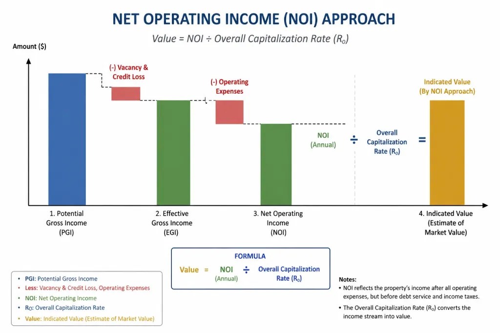
Net Operating Income (NOI) Approach is a traditional theory of capital structure developed by David Durand. This approach argues that the capital structure of a firm is irrelevant and does not affect the overall value of the firm or its weighted average cost of capital (WACC). According to the theory, changes in the proportion of debt and equity financing do not influence the total market value of the company.

The NOI Approach states that although debt is cheaper than equity, any increase in debt financing causes the cost of equity to rise proportionately because shareholders demand higher returns due to increased financial risk. As a result, the overall cost of capital remains constant regardless of the firm’s capital structure.

Definition of Net Operating Income (NOI) Approach

Net Operating Income Approach states that the value of a firm depends on its operating income and business risk, not on its capital structure. Therefore, changes in debt-equity proportions do not affect the firm’s total value or overall cost of capital.

 

Concept of NOI Approach

According to the NOI Approach:

Value of Firm (V)

V = EBIT / Ko

Where:

• V = Total Value of Firm
• EBIT = Earnings Before Interest and Taxes
• Ko = Overall Cost of Capital

Market Value of Equity (S)

S = V − D

Where:

• S = Market Value of Equity
• V = Total Value of Firm
• D = Market Value of Debt

Cost of Equity (Ke)

Ke = NI / S

Where:

• NI = Net Income Available to Equity Shareholders
• S = Market Value of Equity

Example of NOI Approach

Given

• EBIT = ₹3,00,000
• Debt = ₹5,00,000
• Cost of Debt (Kd) = 10%
• Overall Cost of Capital (Ko) = 12%

Step 1: Calculate Value of Firm

V = EBIT / Ko

V = ₹3,00,000 / 0.12

V = ₹25,00,000

Step 2: Calculate Market Value of Equity

S = V − D

S = ₹25,00,000 − ₹5,00,000

S = ₹20,00,000

Step 3: Calculate Interest

Interest = ₹5,00,000 × 10%

Interest = ₹50,000

Step 4: Calculate Net Income

NI = EBIT − Interest

NI = ₹3,00,000 − ₹50,000

NI = ₹2,50,000

Step 5: Calculate Cost of Equity

Ke = NI / S

Ke = ₹2,50,000 / ₹20,00,000

Ke = 12.5%

Answer

• Value of Firm = ₹25,00,000
• Market Value of Equity = ₹20,00,000
• Cost of Equity = 12.5%
• Overall Cost of Capital = 12% (Constant)

Features of Net Operating Income (NOI) Approach

• Capital Structure is Irrelevant

A key feature of the Net Operating Income (NOI) Approach is that capital structure does not affect the value of the firm. According to this theory, whether a company finances its operations through debt, equity, or a combination of both, the total value of the firm remains unchanged. Investors focus on the firm’s earning capacity and business risk rather than its financing pattern. Therefore, changes in leverage do not create additional value. This feature forms the foundation of the NOI Approach and distinguishes it from theories that consider capital structure relevant to firm valuation.

• Value of the Firm Depends on Operating Income

The NOI Approach states that the value of a firm is determined by its operating income, particularly Earnings Before Interest and Taxes (EBIT). The firm’s earning power and business performance are considered the primary factors influencing its market value. Financing decisions do not alter the company’s operating income; therefore, they do not affect firm value. A company with higher and stable operating income will generally have a higher valuation. This feature emphasizes that operational efficiency and profitability are more important than financing choices in determining the overall worth of a business.

• Overall Cost of Capital Remains Constant

According to the NOI Approach, the overall cost of capital (Ko) remains constant regardless of changes in the debt-equity ratio. Even if a company increases its use of debt financing, the weighted average cost of capital does not decline. This occurs because any benefit obtained from cheaper debt is exactly offset by an increase in the cost of equity. As a result, the firm’s overall capitalization rate remains unchanged. This feature supports the idea that leverage does not influence firm value and that financing decisions have no effect on the company’s total cost of capital.

• Cost of Equity Increases with Leverage

The NOI Approach recognizes that higher debt financing increases financial risk for equity shareholders. As leverage rises, shareholders face greater uncertainty because debt holders have a prior claim on earnings. To compensate for this additional risk, equity investors demand a higher rate of return. Therefore, the cost of equity increases proportionately with leverage. This increase offsets the advantage of lower-cost debt financing. This feature reflects the relationship between financial risk and shareholder expectations and explains why the overall cost of capital remains constant despite changes in capital structure.

• Cost of Debt Remains Constant

Another important feature of the NOI Approach is the assumption that the cost of debt remains constant at all levels of leverage. Lenders are assumed to charge the same interest rate regardless of the amount of debt used by the company. Although this assumption may not be realistic in practice, it simplifies the analysis of capital structure. Since the cost of debt remains unchanged, the entire adjustment to increased leverage occurs through a rise in the cost of equity. This feature helps explain the mechanism through which the overall cost of capital remains constant.

• No Optimum Capital Structure Exists

Under the NOI Approach, there is no optimum capital structure because changes in debt and equity proportions do not affect firm value or overall cost of capital. Since leverage neither increases nor decreases the total value of the firm, no particular financing mix is considered superior. Managers cannot create additional value simply by altering the debt-equity ratio. This feature contrasts sharply with the Net Income Approach, which suggests that an optimum capital structure exists. The NOI theory therefore supports the view that financing decisions are irrelevant to maximizing firm value.

• Focuses on Business Risk Rather Than Financial Risk

The NOI Approach emphasizes business risk as the primary determinant of firm value. Business risk arises from the nature of the company’s operations, industry conditions, competition, and economic environment. While financial risk increases with leverage, the theory assumes that investors adjust their required returns accordingly. As a result, firm value continues to depend mainly on operating performance rather than financing decisions. This feature highlights the importance of managerial efficiency, profitability, and operational stability in determining market value, reinforcing the theory’s focus on the earning power of the firm.

• Supports Capital Structure Irrelevance Theory

A significant feature of the NOI Approach is its support for the concept of capital structure irrelevance. The theory argues that investors cannot gain additional wealth merely because a firm changes its financing pattern. Since the overall cost of capital remains constant and firm value is unaffected by leverage, capital structure decisions do not influence shareholder wealth. This idea later influenced modern financial theories, particularly the Modigliani-Miller propositions. As a result, the NOI Approach occupies an important place in financial management by providing a theoretical foundation for understanding the relationship between leverage and firm value.

Assumptions of the NOI Approach

1. Overall Capitalization Rate Remains Constant

The NOI Approach assumes that the overall capitalization rate, also known as the overall cost of capital or Ko, remains constant regardless of the degree of leverage employed by the firm. This means that no matter how the company structures its financing between debt and equity, the market always values the firm by capitalizing its net operating income at the same fixed rate. This constant capitalization rate implies that the total market value of the firm is determined solely by its earning power and operating income, not by its financing decisions, making capital structure completely irrelevant to overall firm valuation under this theoretical framework.

2. Cost of Equity Rises with Increasing Leverage

Unlike the NI Approach, the NOI Approach explicitly recognizes that equity shareholders are rational investors who perceive and respond to increasing financial risk as leverage rises. As the proportion of debt in the capital structure increases, the fixed interest obligations create greater earnings volatility and higher financial risk for equity holders. Consequently, shareholders demand a progressively higher rate of return to compensate for this increased risk, causing the cost of equity to rise proportionally with leverage. This rise in equity cost precisely offsets the benefit of using cheaper debt, ensuring that the overall weighted average cost of capital remains unchanged regardless of the debt-equity mix.

3. Cost of Debt Remains Constant

The NOI Approach assumes that the cost of debt remains constant at all levels of leverage, reflecting the idea that debt holders maintain a prior claim on the firm’s assets and earnings, shielding them from the financial risk of moderate leverage levels. Since debt holders enjoy priority in repayment and their returns are fixed through contractual interest obligations, they do not demand higher returns as the company takes on additional debt within reasonable limits. This constant cost of debt, combined with the rising cost of equity, ensures that the overall capitalization rate remains stable as the firm shifts its financing mix between debt and equity.

4. No Corporate Taxes

Similar to the NI Approach, the basic NOI Approach assumes a taxation-free environment, meaning that corporate income taxes do not exist and therefore the tax-deductibility benefit of interest payments on debt is not considered. In a world without taxes, debt loses its additional advantage of generating a tax shield, making the theoretical argument for capital structure irrelevance more straightforward and internally consistent. This assumption eliminates a significant real-world advantage of debt financing, allowing the model to demonstrate that the only cost benefit of debt, its lower rate, is entirely offset by the rise in equity cost, leaving total firm value and overall cost of capital unaffected by leverage.

5. The Market Values the Firm as a Whole

A fundamental assumption of the NOI Approach is that investors and the market value the firm as a total entity based on its overall earning power and net operating income stream, rather than separately valuing the individual components of its capital structure. This holistic valuation perspective means that the split of total firm value between debt and equity is considered inconsequential, as the market focuses on the overall cash generating ability of the business rather than how those cash flows are divided among different capital providers. Consequently, any restructuring of the financing mix merely redistributes the existing total value between debt holders and shareholders without changing the aggregate firm value.

6. Investors Have Homogeneous Expectations

The NOI Approach assumes that all investors share identical expectations regarding the firm’s future net operating income, overall risk profile, and growth prospects. This homogeneity of expectations ensures that all market participants agree on the appropriate overall capitalization rate to apply when valuing the firm’s earnings stream. Without this assumption, different investors might assign different values to the same firm based on varying perceptions of risk arising from leverage, potentially disrupting the clean theoretical conclusion that capital structure is irrelevant. Homogeneous expectations simplify the model by ensuring consistent market-wide agreement on firm valuation, regardless of the debt-equity composition chosen by management.

Capital Structure under the NOI Approach:

1. Capital Structure is Irrelevant to Firm Value

The most fundamental proposition of the NOI Approach regarding capital structure is that the total market value of a firm is completely independent of its financing mix, making capital structure decisions entirely irrelevant to overall firm valuation. According to this approach, the market values the firm solely based on its net operating income and the overall capitalization rate, both of which remain unaffected by how the firm chooses to divide its financing between debt and equity. Whether a firm uses no debt or substantial leverage, its total market value remains unchanged. Any attempt to increase firm value by substituting equity with cheaper debt is self-defeating, as the resulting rise in equity cost exactly neutralizes the apparent benefit of cheaper debt financing.

2. No Optimal Capital Structure Exists

Unlike the NI Approach, which identifies maximum leverage as the optimal point, the NOI Approach concludes that no single optimal capital structure exists for any firm. Since the overall cost of capital remains constant at every possible debt-equity ratio, there is no particular financing mix that minimizes WACC or maximizes firm value. Every capital structure is equally good or equally bad from a valuation perspective, as changing the proportion of debt and equity merely redistributes value between debt holders and shareholders without altering total firm value. This conclusion challenges the traditional notion that finance managers can enhance firm value through careful capital structure engineering, suggesting that managerial effort is better focused on improving operating performance rather than financing decisions.

3. Cost of Equity Adjusts to Keep WACC Constant

A central mechanism underlying the NOI Approach’s capital structure conclusion is that the cost of equity automatically adjusts upward as leverage increases, precisely offsetting the benefit of incorporating cheaper debt into the capital structure. As the firm takes on more debt, equity shareholders perceive greater financial risk arising from fixed interest obligations and the increased probability of earnings volatility. Rational investors respond by demanding a higher required rate of return on their equity investment to compensate for this additional risk. This systematic rise in equity cost ensures that the weighted average of debt and equity costs, that is WACC, remains constant at all leverage levels, preventing any capital structure change from altering the firm’s overall cost of capital.

4. Market Value of the Firm is Determined by NOI

Under the NOI Approach, the total market value of the firm is determined exclusively by capitalizing the firm’s net operating income at the constant overall capitalization rate, completely independent of the capital structure chosen. The formula used is Total Market Value of Firm = Net Operating Income divided by Overall Capitalization Rate. Since both net operating income and the capitalization rate are unaffected by leverage decisions, the resulting total firm value remains fixed regardless of the debt-equity mix employed. The individual values of debt and equity components may change as the financing mix changes, but their combined total always remains the same, confirming the irrelevance of capital structure to aggregate firm valuation under this approach.

5. Graphical Representation of Capital Structure Irrelevance

When the NOI Approach is represented graphically with the degree of leverage on the horizontal axis, the overall cost of capital curve appears as a perfectly horizontal straight line at a constant level, indicating that WACC does not change regardless of how much debt the firm uses. Simultaneously, the cost of equity curve slopes upward as leverage increases, reflecting the rising financial risk premium demanded by shareholders, while the cost of debt curve remains flat. The horizontal WACC line powerfully illustrates the core conclusion of the NOI Approach, that no capital structure decision can move the overall cost of capital up or down, reinforcing the irrelevance proposition through clear visual representation.

6. Practical Implications of the NOI Approach

Although the NOI Approach concludes that capital structure is theoretically irrelevant, it carries important practical implications for financial managers. It suggests that firms should not waste resources or management attention attempting to find a mythical optimal debt-equity ratio, as no such ratio genuinely exists under this framework. Instead, management should focus on decisions that directly improve operating performance, revenue generation, cost efficiency, and investment returns, since these are the true drivers of firm value. The approach also highlights the importance of investor rationality and market efficiency, reminding managers that sophisticated investors will see through superficial capital restructuring exercises and price the firm based on its fundamental earning power rather than its financing arrangement.

Advantages of the NOI Approach

• Simplicity and Practical Applicability

The NOI Approach offers remarkable conceptual simplicity, making it highly practical for financial managers. It posits that the overall cost of capital (WACC) and firm value remain constant regardless of the debt-equity mix, assuming no taxes and perfect markets. This straightforward framework allows managers to focus on operational efficiency rather than getting entangled in complex capital structure optimization calculations. Unlike the Net Income Approach, which requires intricate computations of changing equity costs, the NOI model provides a clean, easy-to-understand baseline. Practitioners can use this as a starting point for strategic decisions without excessive mathematical modeling, saving both time and analytical resources.

• Emphasis on Operating Efficiency Over Financing

A fundamental advantage of the NOI Approach is its strategic shift in management focus toward operational excellence rather than financial engineering. Since the theory asserts that firm value depends solely on net operating income and business risk—not on how that income is financed—it encourages managers to concentrate on improving production, sales, marketing, and cost control. This operational orientation fosters sustainable competitive advantages through better products, efficient processes, and market expansion. By de-emphasizing the debt-equity mix, the approach prevents management from wasting energy on fruitless arbitrage between debt and equity, redirecting attention toward genuine value-creating activities.

• Recognition of Market Imperfections (Arbitrage Process)

The NOI Approach uniquely validates the existence of investor-level arbitrage as a equilibrating mechanism in financial markets. According to this theory, if two identical firms with different capital structures trade at different valuations, rational investors will engage in homemade leverage—borrowing personally to purchase equity of the unlevered firm and selling the levered firm’s shares. This arbitrage activity quickly corrects any mispricing, ensuring that market values converge. This built-in self-correction mechanism gives the approach strong intuitive appeal, as it acknowledges that sophisticated investors will not pay a premium for what they can replicate personally, thereby maintaining market efficiency.

• Logical Treatment of Equity Capitalization Rate

The NOI Approach provides a logical, intuitive explanation for the behavior of the equity capitalization rate (Ke). As a firm increases its debt proportion, the financial risk borne by equity shareholders rises proportionately. Consequently, the required rate of return on equity (Ke) increases linearly to exactly offset the benefits of cheaper debt. This elegant inverse relationship ensures that the weighted average cost of capital (WACC) remains perfectly unchanged. This treatment recognizes shareholder psychology realistically—investors rationally demand higher compensation for bearing greater residual risk, and this natural market reaction neutralizes any apparent advantage from substituting debt for equity.

• Foundation for Modern Capital Structure Theories

Despite its restrictive assumptions, the NOI Approach serves as the intellectual bedrock for contemporary capital structure theories, most notably Modigliani-Miller (M-M) Proposition I. By establishing that leverage does not affect firm value in a no-tax world, it paved the way for further research incorporating taxes, bankruptcy costs, and asymmetric information. Students and practitioners who master the NOI framework gain a critical conceptual lens for understanding trade-off theory, pecking order theory, and signaling models. Without this foundational understanding, modern financial management becomes disjointed; the NOI Approach offers the essential starting point for all advanced capital structure deliberations.

• Encourages Rational Capital Budgeting Decisions

Since the NOI Approach asserts a constant WACC irrespective of leverage, it allows financial managers to evaluate investment projects using a stable, unchanging discount rate. This consistency eliminates the complex, iterative calculations required to adjust hurdle rates for varying debt proportions across different projects. Managers can therefore focus purely on the project’s operating cash flows and risk characteristics rather than worrying about how the project will be financed. This separation of investment and financing decisions (the famous “separation theorem”) streamlines capital budgeting, reduces computational errors, and ensures that projects are evaluated on their fundamental economic merits alone.

• Neutralizes Unproductive Tax Arbitrage Arguments

In its pure form (assuming no corporate taxes), the NOI Approach effectively neutralizes the temptation for firms to engage in unproductive tax-driven arbitrage through excessive leverage. By demonstrating that the value of the firm remains invariant to the debt-equity mix, it discourages management from taking on dangerous debt levels simply to exploit interest tax shields. This conservative implication protects firms from over-leveraging, which in the real world leads to financial distress, agency conflicts, and bankruptcy. Thus, the approach implicitly advocates for prudent, moderate leverage policies rather than aggressive, high-risk financial structures that could destabilize the enterprise during economic downturns.

Limitations of the NOI Approach

• Assumes Constant Overall Cost of Capital

The NOI approach assumes that the overall cost of capital remains constant regardless of changes in the capital structure. In reality, increasing debt raises the financial risk of the company, causing both the cost of debt and the cost of equity to change. Investors demand higher returns as risk increases. Therefore, the assumption of a constant overall cost of capital is unrealistic and does not reflect actual market conditions. This limitation reduces the practical applicability of the NOI approach in making financing decisions for modern business organizations.

• Ignores Financial Risk

The NOI approach assumes that increasing debt does not affect the firm’s financial risk. However, excessive borrowing increases fixed interest obligations and the possibility of financial distress. As debt rises, shareholders face greater risk because earnings become more uncertain. Consequently, investors demand higher returns on equity. By ignoring the impact of financial risk, the NOI approach fails to represent the real relationship between leverage and the cost of capital. This makes the approach less suitable for practical financial management and capital structure planning.

• Unrealistic Assumption of Perfect Capital Market

The NOI approach is based on the assumption of a perfect capital market where there are no taxes, transaction costs, or information differences among investors. In practice, capital markets are imperfect due to taxes, brokerage charges, government regulations, and unequal access to information. These market imperfections influence financing decisions and affect the cost of capital. Since the assumptions of the NOI approach rarely exist in the real business environment, its conclusions may not accurately represent actual corporate financing situations.

• Ignores Tax Benefits of Debt

The NOI approach assumes that debt financing does not provide any tax advantage. In reality, interest paid on debt is generally tax deductible, reducing the company’s taxable income and lowering the effective cost of debt. This tax shield makes debt financing more attractive than equity in many situations. By ignoring the tax benefits associated with borrowing, the NOI approach underestimates the value of debt financing and provides an incomplete explanation of capital structure decisions in modern financial management.

• Assumes Cost of Debt Remains Constant

According to the NOI approach, the cost of debt remains unchanged regardless of the amount of borrowing. In practice, lenders charge higher interest rates when a company’s debt level increases because the risk of default becomes greater. As financial leverage rises, the cost of debt usually increases rather than remaining constant. This unrealistic assumption weakens the practical usefulness of the NOI approach and limits its ability to explain the actual behaviour of borrowing costs in competitive financial markets.

• Difficult to Apply in Practice

The assumptions of the NOI approach are highly theoretical and difficult to apply in real business situations. Market conditions, investor expectations, interest rates, taxes, and business risks continuously change over time. As a result, the cost of debt, cost of equity, and overall cost of capital rarely remain constant. Finance managers must consider these changing factors while making capital structure decisions. Therefore, the NOI approach provides only a simplified theoretical framework and has limited practical application in financial management.

• Overlooks Investor Behaviour

The NOI approach assumes that investors are rational and react uniformly to changes in the company’s capital structure. However, investor decisions are influenced by factors such as market sentiment, expectations, risk perception, and economic conditions. Different investors may value the same company differently based on their individual preferences and investment objectives. By overlooking these behavioural factors, the NOI approach fails to explain how investor attitudes can influence the market value of the firm and its financing decisions.

• Limited Practical Acceptance

The NOI approach has limited acceptance in modern financial management because its assumptions do not match real business conditions. Financial decisions today are influenced by taxes, bankruptcy costs, agency costs, market imperfections, and changing investor expectations. Modern capital structure theories provide more realistic explanations by considering these practical factors. Although the NOI approach is important for understanding the theoretical relationship between capital structure and firm value, it is mainly useful for academic study rather than practical financial decision making.

Net Income Approach, propounded by David Durand, suggests that a firm’s capital structure decision is relevant to its overall valuation and cost of capital. According to this approach, a firm can increase its total value and reduce its overall cost of capital by increasing the proportion of debt in its capital structure, since debt is generally a cheaper source of financing compared to equity. As the degree of leverage increases, the Weighted Average Cost of Capital decreases, leading to an increase in the market value of the firm. This approach assumes that both the cost of debt and cost of equity remain constant regardless of changes in the leverage level.

Definition of Net Income Approach

Net Income Approach states that the value of a firm can be increased and the overall cost of capital can be reduced by increasing the proportion of debt in the capital structure, assuming the costs of debt and equity remain constant.

Net Income (NI) Diagram:

• Cost of Equity (Ke) → constant (horizontal red line)
• Cost of Debt (Kd) → constant (horizontal blue line)
• Weighted Average Cost of Capital (WACC) → decreases as leverage increases (downward-sloping green line)

Concept of Net Income Approach

According to the NI Approach:

Value of Firm (V)

V = S + D

Where:

• V = Total Value of Firm
• S = Market Value of Equity
• D = Market Value of Debt

Cost of Equity

Ke = NI / S

Where:

• NI = Net Income Available to Equity Shareholders
• S = Market Value of Equity

Overall Cost of Capital

Ko = EBIT / V

Where:

• Ko = Overall Cost of Capital
• EBIT = Earnings Before Interest and Taxes
• V = Total Value of Firm

Example of Net Income Approach

Given

• EBIT = ₹2,00,000
• Debt = ₹5,00,000
• Cost of Debt (Kd) = 10%
• Cost of Equity (Ke) = 15%

Step 1: Calculate Interest

Interest = ₹5,00,000 × 10%

= ₹50,000

Step 2: Calculate Net Income

Net Income = EBIT − Interest

= ₹2,00,000 − ₹50,000

= ₹1,50,000

Step 3: Calculate Market Value of Equity

S = NI / Ke

= ₹1,50,000 / 0.15

= ₹10,00,000

Step 4: Calculate Total Value of Firm

V = S + D

= ₹10,00,000 + ₹5,00,000

= ₹15,00,000

Step 5: Calculate Overall Cost of Capital

Ko = EBIT / V

= ₹2,00,000 / ₹15,00,000

= 13.33%

Answer

• Market Value of Equity = ₹10,00,000
• Total Value of Firm = ₹15,00,000
• Overall Cost of Capital = 13.33%

Assumptions of the NI Approach

1. Cost of Debt Remains Constant

The NI Approach assumes that the cost of debt remains constant and unaffected regardless of the degree of leverage employed by the firm. This means that as the company increases its borrowing, lenders do not demand a higher interest rate to compensate for the increased financial risk associated with higher debt levels. In reality, as debt increases, the risk of default rises, and creditors typically require higher returns to compensate for this added risk. However, this approach simplifies the analysis by holding the cost of debt fixed, allowing the focus to remain solely on how the debt-equity mix affects overall valuation.

2. Cost of Equity Remains Constant

Similarly, the NI Approach assumes that the cost of equity remains unchanged irrespective of how much debt the firm takes on. This implies that shareholders do not perceive any additional financial risk from increased leverage and therefore do not demand a higher rate of return as the company’s debt proportion rises. In practical scenarios, increased debt typically heightens the financial risk borne by equity shareholders due to fixed interest obligations, which would normally lead to a higher required return on equity. This assumption isolates the effect of capital structure on firm value by holding the equity cost constant throughout the analysis.

3. No Corporate Taxes

The original NI Approach assumes a world without corporate taxes, meaning that the tax-deductibility benefit of interest payments on debt is not considered in the analysis. This assumption simplifies the model by ignoring the tax shield advantage that debt financing typically provides in real-world scenarios, where interest expense reduces taxable income and lowers the effective cost of debt. Without this assumption, the conclusion that increasing leverage always reduces the overall cost of capital might be even more pronounced due to the additional tax benefits, but the basic NI Approach intentionally excludes this factor for analytical simplicity.

4. Cost of Debt is Less Than Cost of Equity

A fundamental assumption underlying the NI Approach is that the cost of debt is always lower than the cost of equity, since debt holders bear lower risk than equity shareholders due to their priority claim on assets and fixed, contractual returns. This cost differential is the primary driver behind the conclusion that increasing the proportion of debt in the capital structure reduces the overall weighted average cost of capital. Without this assumption that debt is cheaper, the entire premise of the NI Approach, that leverage enhances firm value, would not hold true within the theoretical framework presented.

5. No Change in Investors’ Risk Perception

The NI Approach assumes that investors, both debt holders and equity shareholders, do not alter their risk perception of the firm as its degree of financial leverage increases. This means the market does not penalize the company with higher required returns despite the increased financial risk associated with higher fixed interest obligations. In actual capital markets, investors are generally risk-averse and tend to demand higher compensation as leverage rises due to increased bankruptcy risk and earnings volatility. This unrealistic assumption is a major criticism of the approach, as it does not reflect rational investor behavior in efficient markets.

6. The Firm Has a 100% Dividend Payout Ratio

The NI Approach assumes that the firm distributes all of its earnings as dividends to shareholders, with no retained earnings kept within the business for reinvestment purposes. This simplifies the valuation process by ensuring that the net income available to equity shareholders directly translates into dividend payments, making it easier to calculate the market value of equity using the capitalization rate. This assumption avoids complications that would arise from retained earnings affecting future growth, earnings per share, or stock valuation, allowing the model to focus purely on the immediate relationship between capital structure and firm value.

Optimum Capital Structure under the NI Approach

1. Maximum Leverage as the Optimal Point

According to the Net Income Approach, the optimum capital structure is achieved at the point of maximum possible debt, theoretically approaching 100% debt financing. Since the cost of debt is assumed to remain constant and lower than the cost of equity at all levels of leverage, every additional unit of debt replacing equity continuously reduces the overall Weighted Average Cost of Capital. Consequently, the approach concludes that there is no single moderate optimal debt-equity ratio; instead, firm value keeps rising indefinitely as leverage increases, with the theoretical optimum lying at the extreme point where the firm relies almost entirely on debt capital.

2. Continuous Decline in WACC with Increasing Leverage

As the proportion of debt in the capital structure rises, the overall cost of capital declines steadily because debt, being cheaper than equity, pulls down the weighted average. Since both individual component costs, debt and equity, are assumed constant under this approach, there is no offsetting increase in cost to counteract the benefit of higher leverage. This creates a straight, downward-sloping WACC curve as leverage increases, reinforcing the conclusion that the firm should continuously substitute equity with debt to minimize its overall cost of capital and thereby maximize its market value at every incremental stage of borrowing.

3. Corresponding Increase in Market Value of the Firm

As WACC continuously decreases with rising leverage, the market value of the firm correspondingly increases, since firm value under this approach is calculated by capitalizing the net operating income at the declining overall cost of capital. This inverse relationship between WACC and firm value means that as debt is added, the present value of the firm’s future earnings stream rises. Under the NI Approach, this increase in value continues without limit as leverage rises, theoretically suggesting that firm value is maximized only when the company is financed almost entirely through debt rather than equity capital.

4. No Realistic Trade-Off Point Identified

Unlike more balanced theories of capital structure, the NI Approach does not identify a realistic trade-off point where the benefits of cheap debt are offset by rising financial risk. Since the cost of equity is assumed unaffected by leverage, there is no rising risk premium to counterbalance the advantage of cheaper debt at higher leverage levels. This means the approach fails to capture a genuine optimal balance between debt and equity that reflects real-world risk considerations, making its conclusion of “more debt is always better” a theoretical extreme rather than a practically achievable or sustainable capital structure target.

5. Graphical Representation of the Optimum Point

When plotted graphically, with leverage (debt-to-equity ratio) on the horizontal axis and cost of capital or firm value on the vertical axis, the NI Approach shows a continuously declining WACC curve and a continuously rising firm value curve as leverage increases. There is no minimum point on the WACC curve or maximum point on the value curve within the relevant range; both curves move monotonically in their respective directions. This graphical representation visually reinforces the theoretical conclusion that the optimum capital structure lies at the boundary of maximum debt usage, rather than at some interior point of moderate leverage.

6. Practical Unrealism of the Conclusion

While theoretically elegant, the conclusion that 100% debt represents the optimum capital structure is widely criticized as unrealistic and impractical in real-world financial markets. Excessive reliance on debt significantly increases financial risk, bankruptcy probability, and the likelihood of default, which would naturally cause both cost of debt and cost of equity to rise as leverage increases, contradicting the approach’s core assumptions. This limitation highlights why the NI Approach is considered more of a theoretical benchmark for understanding the directional impact of leverage on firm value, rather than a practically applicable guideline for determining actual optimal financing decisions.

Advantages of the NI Approach

Limitations of the NI Approach

• Assumes Constant Cost of Equity

One of the major limitations of the NI Approach is its assumption that the cost of equity remains constant regardless of changes in financial leverage. In reality, as a company increases its debt, equity shareholders face higher financial risk because debt obligations must be paid before dividends. Consequently, shareholders demand a higher rate of return to compensate for this increased risk. Therefore, the cost of equity generally rises with higher leverage. By ignoring this practical reality, the NI Approach presents an unrealistic view of capital structure and may lead to inaccurate conclusions regarding firm value.

• Assumes Constant Cost of Debt

The NI Approach assumes that the cost of debt remains unchanged even when a company significantly increases its borrowings. However, lenders generally perceive highly leveraged firms as riskier and may demand higher interest rates on additional debt. As debt levels increase, the probability of financial distress and default also rises. Consequently, the cost of debt tends to increase rather than remain constant. This unrealistic assumption weakens the practical applicability of the NI Approach because financing costs in real-world situations are influenced by the firm’s risk profile and borrowing capacity.

• Ignores Financial Risk

A significant limitation of the NI Approach is that it ignores the increasing financial risk associated with excessive debt financing. Debt creates fixed obligations in the form of interest and principal repayments. As leverage rises, the risk of financial distress also increases, particularly during periods of declining earnings. The NI Approach assumes that investors and lenders do not react to this increased risk, which is not realistic. By overlooking financial risk, the theory overestimates the benefits of debt financing and fails to provide a balanced assessment of capital structure decisions.

• Unrealistic Assumptions

The NI Approach is based on several assumptions that rarely exist in actual business environments. It assumes constant costs of debt and equity, no taxes, efficient capital markets, and rational investor behavior. In practice, these conditions are seldom met. Market imperfections, taxation, transaction costs, and changing investor expectations significantly affect financing decisions. Because the theory relies heavily on unrealistic assumptions, its conclusions may not accurately reflect real-world corporate finance situations. This limitation reduces its usefulness as a practical guide for determining an optimal capital structure.

• Ignores Corporate Taxes

Another limitation of the NI Approach is that it ignores the impact of corporate taxes on financing decisions. In reality, interest payments on debt are generally tax-deductible, creating a tax shield that reduces the effective cost of debt. Taxes play an important role in determining the attractiveness of debt financing and the overall cost of capital. By excluding taxation from its analysis, the NI Approach fails to capture a key factor influencing capital structure decisions. As a result, its conclusions regarding firm value and financing choices may not accurately represent actual business conditions.

• Promotes Excessive Use of Debt

According to the NI Approach, increasing debt continuously lowers the cost of capital and increases the value of the firm. This conclusion may encourage companies to rely excessively on debt financing. However, excessive debt can create serious financial problems, including higher interest burdens, liquidity difficulties, and bankruptcy risk. In practice, firms cannot increase debt indefinitely without facing adverse consequences. Therefore, the theory’s recommendation of continuous leverage is unrealistic and potentially dangerous. This limitation highlights the need for a more balanced approach to capital structure decisions.

• Limited Practical Applicability

Although the NI Approach provides useful theoretical insights, its practical application is limited. Real-world financing decisions involve numerous factors such as market conditions, investor expectations, business risk, taxation, and regulatory requirements. The approach does not adequately address these complexities. As a result, financial managers rarely rely solely on the NI Approach when making capital structure decisions. Instead, they use more comprehensive models that incorporate risk, taxation, and market behavior. Therefore, the NI Approach serves primarily as a theoretical concept rather than a practical financial management tool.

• Overlooks Market Reactions

The NI Approach assumes that investors and lenders do not change their behavior as a company’s leverage increases. In reality, financial markets respond to changes in risk. Investors may demand higher returns, lenders may increase interest rates, and credit ratings may decline when debt levels become excessive. These market reactions significantly affect a firm’s financing costs and value. By ignoring the dynamic relationship between leverage and market perception, the NI Approach oversimplifies capital structure decisions. Consequently, it may produce results that differ substantially from actual outcomes observed in financial markets.

Beta (β) is a measure of the systematic risk of a company’s stock in relation to the overall market. It indicates how sensitive a company’s returns are to changes in market returns. However, a company’s beta is influenced not only by its business risk but also by its financial risk arising from the use of debt financing.

To separate these risks, financial analysts use the concepts of Unlevering Beta and Relevering Beta.

1. Unlevering Beta (Asset Beta)

Unlevering Beta, also known as Asset Beta, is the process of removing the effect of financial leverage (debt) from a company’s equity beta. The resulting beta reflects only the business risk of the company’s assets and operations, excluding the additional risk created by debt financing.

Since different companies use different amounts of debt in their capital structures, comparing their equity betas directly may be misleading. Unlevering beta eliminates the impact of financial risk and provides a common basis for comparison. Therefore, Asset Beta represents the true operating risk of a company and is widely used in valuation, mergers and acquisitions, capital budgeting, and investment analysis.

Definition

Unlevered Beta is the beta that measures the risk of a company’s assets without considering the effects of debt financing. It reflects only the business risk associated with the company’s operations.

Formula of Unlevering Beta

βU = βL / [1 + (1 − T) (D/E)]

Where:

• βU = Unlevered Beta (Asset Beta)
• βL = Levered Beta (Equity Beta)
• T = Corporate Tax Rate
• D = Market Value of Debt
• E = Market Value of Equity

Calculation of Unlevering Beta

Example 1

Given:

• Levered Beta = 1.50
• Debt = ₹400 lakh
• Equity = ₹600 lakh
• Tax Rate = 30%

Step 1: Calculate Debt-Equity Ratio

D/E = 400 / 600 = 0.667

Step 2: Apply Formula

βU = 1.50 / [1 + (1 − 0.30)(0.667)]

βU = 1.50 / [1 + 0.467]

βU = 1.50 / 1.467

βU = 1.02

Answer

Unlevered Beta = 1.02

This beta represents only the business risk of the company’s assets.

Example 2

Given:

• Levered Beta = 1.80
• Debt = ₹500 lakh
• Equity = ₹1,000 lakh
• Tax Rate = 25%

Solution

D/E = 500 / 1000 = 0.50

βU = 1.80 / [1 + (1 − 0.25)(0.50)]

βU = 1.80 / 1.375

βU = 1.31

Answer

Asset Beta = 1.31

Components of Unlevering Beta (Asset Beta)

• Levered Beta (Equity Beta)

Levered Beta, also known as Equity Beta, is the starting point in the process of unlevering beta. It measures the total risk faced by equity shareholders, including both business risk and financial risk arising from debt financing. Since companies often use borrowed funds, the equity beta reflects the impact of leverage on shareholder returns. During unlevering, this beta is adjusted to remove the influence of debt and isolate business risk. Therefore, levered beta is a crucial component because it provides the base value from which the asset beta is derived.

• Market Value of Debt (D)

The market value of debt represents the total value of the company’s long-term borrowings, debentures, bonds, and loans. Debt increases financial leverage and consequently increases the risk borne by equity shareholders. In the unlevering process, the amount of debt is considered to determine how much financial risk is embedded in the equity beta. A higher level of debt generally results in a greater difference between levered beta and unlevered beta. Therefore, the market value of debt is an essential component for accurately separating financial risk from business risk.

• Market Value of Equity (E)

The market value of equity refers to the total market capitalization of a company, calculated by multiplying the number of outstanding shares by their market price. It represents the ownership value held by shareholders and forms an important part of the debt-equity relationship. During the unlevering process, the market value of equity is used along with debt to calculate the debt-equity ratio. This ratio helps determine the extent to which financial leverage influences shareholder risk. Therefore, market value of equity plays a significant role in deriving the company’s true business risk.

• Debt-Equity Ratio (D/E Ratio)

The Debt-Equity Ratio is a key component in the unlevering beta formula. It measures the proportion of debt financing relative to shareholders’ equity. This ratio indicates the degree of financial leverage employed by the company. A higher debt-equity ratio signifies greater financial risk and a larger adjustment when converting levered beta into unlevered beta. Conversely, a lower ratio indicates less financial leverage and a smaller adjustment. The debt-equity ratio is critical because it directly determines the extent to which financial risk is removed from the equity beta.

• Corporate Tax Rate (T)

The corporate tax rate is an important component because debt financing provides a tax advantage through the deductibility of interest expenses. The unlevering beta formula incorporates the tax rate to account for this tax shield. A higher tax rate increases the benefit of debt financing and affects the adjustment made to remove financial risk. By including the tax factor, the formula provides a more realistic measure of business risk. Therefore, the corporate tax rate ensures that the impact of debt is accurately reflected when calculating the unlevered beta.

• Financial Risk

Financial risk is the additional risk borne by shareholders due to the use of debt financing. It arises because debt obligations require fixed interest and principal payments regardless of business performance. Unlevering beta aims to remove this financial risk from the equity beta so that only business risk remains. Understanding financial risk is essential because it explains the difference between levered beta and unlevered beta. The greater the financial risk, the larger the adjustment required. Thus, financial risk serves as a fundamental component in the concept and application of unlevering beta.

• Business Risk

Business risk refers to the uncertainty associated with a company’s core operations, industry conditions, competition, and economic environment. Unlike financial risk, business risk exists regardless of how the company is financed. The primary objective of unlevering beta is to isolate and measure this business risk independently. Asset beta obtained after unlevering reflects only operational risk and excludes the effects of leverage. Since business risk forms the foundation of a company’s overall risk profile, it is one of the most important components in the unlevering beta process.

• Unlevered Beta (Asset Beta)

Unlevered Beta, also called Asset Beta, is the final outcome of the unlevering process. It measures the systematic risk of a company’s assets without considering debt financing. This beta reflects only the business risk associated with the company’s operations and investments. Asset beta is widely used for comparing companies with different capital structures, valuing businesses, and estimating project-specific risks. It serves as a neutral risk measure unaffected by financing decisions. Therefore, unlevered beta is both a component and the ultimate objective of the unlevering process in financial analysis.

2. Relevering Beta (Equity Beta)

Relevering Beta is the process of adjusting an unlevered beta (asset beta) to reflect the impact of a specific or target capital structure. It involves adding the effect of financial leverage (debt) back to the asset beta to determine the Equity Beta (Levered Beta). While unlevered beta measures only business risk, relevered beta measures both business risk and financial risk.

Relevering beta is commonly used in corporate valuation, mergers and acquisitions, capital budgeting, and CAPM calculations. It helps analysts estimate the risk faced by equity shareholders when a company uses debt financing. Since different capital structures create different levels of financial risk, relevering beta provides a more realistic measure of shareholder risk under a specific financing arrangement.

Definition

Relevering Beta is the process of adjusting asset beta to incorporate the effect of debt financing and obtain the equity beta that reflects both business and financial risk.

Formula of Relevering Beta

βL = βU × [1 + (1 − T)(D/E)]

Where:

• βL = Levered Beta (Equity Beta)
• βU = Unlevered Beta (Asset Beta)
• T = Corporate Tax Rate
• D = Market Value of Debt
• E = Market Value of Equity

Calculation of Relevering Beta

Example 1

Given:

• Unlevered Beta = 1.10
• Debt = ₹400 lakh
• Equity = ₹500 lakh
• Tax Rate = 30%

Step 1: Calculate Debt-Equity Ratio

D/E = 400 / 500 = 0.80

Step 2: Apply Formula

βL = 1.10 × [1 + (1 − 0.30)(0.80)]

βL = 1.10 × [1 + 0.56]

βL = 1.10 × 1.56

βL = 1.72

Answer

Relevered Beta (Equity Beta) = 1.72

Example 2

Given:

• Asset Beta = 0.95
• Debt = ₹600 lakh
• Equity = ₹600 lakh
• Tax Rate = 25%

Solution

D/E = 600 / 600 = 1.00

βL = 0.95 × [1 + (1 − 0.25)(1)]

βL = 0.95 × 1.75

βL = 1.66

Answer

Equity Beta = 1.66

Components of Relevering Beta (Equity Beta)

1. Unlevered Beta (Asset Beta)

Unlevered Beta, also known as Asset Beta, is the foundation of the relevering process. It measures the systematic risk of a company’s assets without considering the effects of debt financing. This beta reflects only business risk arising from the company’s operations, industry conditions, and market environment. During relevering, the unlevered beta is adjusted to include financial risk and obtain the equity beta. Since it serves as the starting point for the calculation, its accuracy is crucial. A higher unlevered beta indicates greater operational risk, which ultimately influences the resulting relevered beta.

Example: If Asset Beta = 1.10, this value will be adjusted based on the company’s capital structure to determine Equity Beta.

2. Levered Beta (Equity Beta)

Levered Beta, or Equity Beta, is the final outcome of the relevering process. It measures the total systematic risk borne by equity shareholders, including both business risk and financial risk. When a company uses debt financing, shareholders face additional risk because debt obligations must be paid regardless of profitability. Relevering beta incorporates this risk into the calculation. Equity beta is widely used in CAPM, business valuation, and investment analysis. It helps determine the return expected by shareholders and provides a realistic assessment of shareholder risk under a specific capital structure.

Example: If Asset Beta = 1.10 and leverage increases risk, the resulting Equity Beta may become 1.72.

3. Market Value of Debt (D)

The market value of debt represents the current value of long-term borrowings, bonds, debentures, and loans used by the company. Debt financing increases financial leverage and therefore raises the risk faced by equity shareholders. During the relevering process, the amount of debt determines how much additional financial risk is added to the asset beta. A higher debt level generally results in a higher equity beta. Therefore, the market value of debt is an important component because it directly influences the magnitude of leverage and the overall risk reflected in the relevered beta.

Example: If Debt = ₹500 lakh, it contributes to increasing shareholder risk and affects the relevered beta calculation.

4. Market Value of Equity (E)

The market value of equity refers to the total value of shareholders’ ownership in the company, measured by market capitalization. It is calculated by multiplying the market price per share by the number of outstanding shares. Equity forms the denominator in the debt-equity ratio used during relevering. A larger equity base reduces the impact of debt on financial leverage, while a smaller equity base increases leverage effects. Therefore, the market value of equity is essential in determining the degree of financial risk that is incorporated into the equity beta.

Example

If Equity = ₹1,000 lakh, the leverage effect is lower than when equity is only ₹500 lakh.

5. Debt-Equity Ratio (D/E Ratio)

The Debt-Equity Ratio is one of the most significant components of relevering beta. It measures the proportion of debt financing relative to shareholders’ equity. This ratio determines the extent of financial leverage used by the company. A higher debt-equity ratio means that the company relies more heavily on borrowed funds, increasing financial risk and shareholder exposure. Consequently, the equity beta rises. A lower ratio indicates less leverage and a smaller increase in beta. Thus, the debt-equity ratio plays a critical role in adjusting asset beta to reflect shareholder risk accurately.

Example

If Debt = ₹600 lakh and Equity = ₹600 lakh:

D/E = 600 / 600 = 1

This ratio significantly increases the equity beta.

6. Corporate Tax Rate (T)

The corporate tax rate is included in the relevering beta formula because debt financing provides a tax shield through deductible interest payments. The tax shield reduces the effective cost of debt and influences the impact of leverage on shareholder risk. By incorporating the tax rate, the relevering formula provides a more realistic adjustment to beta. A higher tax rate increases the tax benefit associated with debt and affects the extent to which leverage contributes to risk. Therefore, the corporate tax rate is an essential component for accurately estimating equity beta.

Example

If the corporate tax rate is 30%, the debt adjustment factor becomes:

(1 − 0.30) = 0.70

This factor is applied in the relevering formula.

7. Financial Risk

Financial risk refers to the additional risk borne by shareholders due to the use of debt financing. Unlike business risk, financial risk arises because the company must meet fixed interest and principal repayment obligations. As debt levels increase, shareholders face greater uncertainty regarding returns. Relevering beta incorporates this financial risk into the asset beta, resulting in a higher equity beta. Understanding financial risk is crucial because it explains why companies with similar operations can have different equity betas. Therefore, financial risk is a central component in the relevering process.

Example: A company with substantial debt will generally have a higher equity beta than a debt-free company operating in the same industry.

8. Capital Structure

Capital structure refers to the combination of debt and equity used to finance a company’s assets and operations. It is the ultimate factor influencing the relevered beta because different financing mixes create different levels of financial risk. Relevering beta adjusts asset beta according to a specific capital structure, enabling analysts to estimate shareholder risk under alternative financing scenarios. Companies with aggressive debt financing generally have higher equity betas, while conservatively financed firms have lower equity betas. Thus, capital structure serves as the overall framework within which the relevering process operates.

Example: A company financed with 70% debt and 30% equity will generally have a higher equity beta than a company financed with 20% debt and 80% equity.

Regular Method, also known as the Dividend Yield Method, is one of the simplest methods used to calculate the cost of equity capital. This method assumes that shareholders invest in a company primarily to receive dividends. Therefore, the cost of equity is determined by comparing the annual dividend per share with the current market price of the share.

According to this method, the dividend received by shareholders represents the return expected on their investment. The higher the dividend relative to the market price, the higher will be the cost of equity. The method is particularly suitable for companies that pay stable and regular dividends over time.

Definition of Regular Method (Dividend Yield Method)

The Dividend Yield Method defines the cost of equity capital as the rate of return obtained by dividing the annual dividend per share by the current market price per share.

Formula of Dividend Yield Method

Ke = D / P × 100

Where:

• Ke = Cost of Equity Capital
• D = Annual Dividend per Share
• P = Current Market Price per Share

Features of Regular Method (Dividend Yield Method)

• Based on Dividend Income

The Dividend Yield Method is primarily based on the dividend income received by shareholders. It assumes that dividends are the main source of return for equity investors. The cost of equity is determined by comparing the annual dividend per share with the current market price of the share. Since dividends represent the actual cash return earned by shareholders, this method directly links shareholder expectations with dividend payments. This feature makes the method simple and practical for companies that maintain a consistent dividend policy and regularly distribute profits to shareholders.

• Uses Market Price of Shares

A significant feature of the Dividend Yield Method is the use of the current market price of shares in calculating the cost of equity. The market price reflects investors’ perception of the company’s value and future prospects. By relating dividends to market price, the method determines the return expected by shareholders on their investment. Changes in market price directly affect the calculated cost of equity. This feature ensures that the method considers prevailing market conditions and investor expectations while estimating the return required by equity shareholders.

• Simple and Easy to Calculate

The Dividend Yield Method is one of the simplest methods used for calculating the cost of equity capital. It requires only two pieces of information: annual dividend per share and market price per share. The formula is straightforward and easy to understand, making it suitable for students, investors, and financial managers. Unlike advanced models such as CAPM, it does not involve complex calculations or risk assessments. This simplicity makes the method highly useful for basic financial analysis and quick estimation of shareholder-required returns in dividend-paying companies.

• Suitable for Stable Dividend-Paying Companies

This method is particularly appropriate for companies that have a stable and regular dividend policy. When dividends are paid consistently over time, the method can provide a reasonable estimate of the cost of equity capital. Companies with predictable earnings and established dividend records are ideal candidates for this approach. However, the method becomes less reliable when dividend payments fluctuate significantly. Therefore, its effectiveness largely depends on the stability and consistency of dividend distributions made by the company to its shareholders.

• Focuses on Shareholder Returns

The Dividend Yield Method directly focuses on the return expected by equity shareholders. Since shareholders invest funds with the expectation of receiving dividends, the method measures the cost of equity from their perspective. It helps management understand the minimum return required to satisfy investors and maintain shareholder confidence. This feature makes the method useful for evaluating financing decisions and determining the attractiveness of equity investments. By emphasizing shareholder returns, the method supports financial planning and contributes to shareholder wealth maximization objectives.

• Does Not Consider Growth in Dividends

A notable feature of the Regular Method is that it considers only the current dividend and ignores future growth in dividend payments. The calculation assumes that dividends remain constant over time and does not account for potential increases resulting from higher profits or business expansion. This feature simplifies the method but may reduce its accuracy in growing companies. As a result, the calculated cost of equity may be lower than the actual return expected by shareholders. Therefore, the method is more suitable for firms with stable rather than rapidly growing dividends.

• Traditional Approach to Cost of Equity

The Dividend Yield Method is regarded as one of the oldest and most traditional approaches for estimating the cost of equity capital. Before the development of modern risk-based models, this method was widely used by financial managers and investors. Its popularity stemmed from its simplicity and reliance on easily available information. Although more sophisticated methods are now available, the Dividend Yield Method continues to be taught and used for basic financial analysis. This traditional nature makes it an important foundation for understanding the concept of cost of equity.

• Limited Consideration of Risk Factors

Another important feature of the Dividend Yield Method is that it does not explicitly consider investment risk. Unlike CAPM, which incorporates systematic risk through the beta coefficient, this method focuses only on dividends and market price. As a result, differences in business risk, market volatility, and economic conditions are not reflected in the calculation. While this simplicity is advantageous, it may also reduce the accuracy of the estimated cost of equity. Therefore, the method is best used when risk considerations are relatively stable or when a basic estimate is sufficient.

Components of Regular Method (Dividend Yield Method)

Regular Method (Dividend Yield Method) calculates the cost of equity capital by relating the annual dividend paid to shareholders with the current market price of the share. The formula is:

Ke = D / P × 100

Where:

• Ke = Cost of Equity Capital
• D = Annual Dividend per Share
• P = Market Price per Share

The effectiveness of this method depends on its key components. Each component plays an important role in determining the return expected by equity shareholders.

1. Annual Dividend per Share (D)

Annual Dividend per Share is the amount of profit distributed by a company to each equity shareholder during a financial year. It represents the direct cash return received by investors on their investment. In the Dividend Yield Method, the dividend is considered the primary source of shareholder return. A higher dividend generally results in a higher cost of equity, assuming the market price remains unchanged.

Example

Suppose a company declares an annual dividend of ₹12 per share.

Then:

D = ₹12

If the market price is ₹150:

Ke = 12 / 150 × 100

Ke = 8%

Thus, the dividend directly influences the cost of equity calculation.

2. Current Market Price per Share (P)

The current market price per share is the price at which a company’s share is trading in the stock market. It reflects investor expectations, company performance, market conditions, and future growth prospects. In the Dividend Yield Method, the market price represents the amount invested by shareholders to earn dividend income.

A higher market price reduces the dividend yield and therefore lowers the cost of equity, while a lower market price increases the dividend yield.

Example

Dividend per Share = ₹10

Market Price = ₹125

Ke = 10 / 125 × 100

Ke = 8%

If the market price falls to ₹100:

Ke = 10 / 100 × 100

Ke = 10%

This shows the importance of market price in determining shareholder returns.

3. Dividend Yield

Dividend yield is the percentage return that shareholders receive from dividends relative to the market price of the share. It forms the basis of the Dividend Yield Method and indicates the earning power of a share from dividend payments alone.

The dividend yield helps investors compare the returns offered by different companies and assess the attractiveness of equity investments. It serves as a measure of the return expected by shareholders under this method.

Example

Dividend per Share = ₹15

Market Price = ₹200

Dividend Yield = 15 / 200 × 100

Dividend Yield = 7.5%

Therefore, shareholders earn a dividend return of 7.5% on their investment.

4. Shareholder Expected Return

The Dividend Yield Method assumes that shareholders primarily expect returns through dividend payments. Therefore, shareholder expected return is an important component of the method. The calculated dividend yield is treated as the return required by investors for investing in the company’s equity shares.

This expected return serves as the company’s cost of equity capital because it represents the minimum return needed to satisfy shareholders and maintain the market value of shares.

Example

If shareholders receive a dividend yield of 9%, the company must earn at least 9% on equity-financed investments to meet shareholder expectations.

5. Stable Dividend Policy

A stable dividend policy is an important component underlying the Dividend Yield Method. The method works effectively only when a company pays dividends regularly and consistently. Stable dividends allow investors to estimate future returns more accurately and make the cost of equity calculation more reliable.

Companies with irregular dividend payments may produce misleading results because dividend yield can fluctuate significantly from year to year.

Example

A company consistently pays dividends of ₹8, ₹8.5, ₹9, and ₹9.5 over four years.

Such stability makes the Dividend Yield Method more applicable and reliable for estimating the cost of equity.

6. Equity Share Capital

The Dividend Yield Method specifically focuses on equity share capital because dividends are paid only to equity shareholders after meeting all other financial obligations. Equity shareholders bear the highest level of risk and therefore expect returns through dividend income and capital appreciation.

This component emphasizes that the method is designed exclusively for estimating the cost of equity and not the cost of debt or preference shares.

Example

A company has:

• Equity Share Capital = ₹50,00,000
• Dividend Rate = 10%

The dividends distributed to equity shareholders become the basis for calculating the cost of equity using this method.

7. Market Valuation of Shares

Market valuation reflects how investors assess a company’s performance, profitability, and future growth prospects. Since the Dividend Yield Method uses the market price of shares, market valuation becomes an indirect but important component.

A company with strong investor confidence generally has a higher market price, resulting in a lower dividend yield. Conversely, lower market valuation increases the dividend yield and cost of equity.

Example

Dividend = ₹10

Company A Market Price = ₹200

Ke = 5%

Company B Market Price = ₹100

Ke = 10%

Thus, market valuation directly influences the estimated cost of equity.

8. Relationship Between Dividend and Investment Value

The core principle of the Dividend Yield Method is the relationship between dividend income and the amount invested in purchasing shares. This relationship determines the rate of return expected by shareholders and forms the foundation of the method.

The method assumes that investors evaluate their returns by comparing the dividend received with the investment made in acquiring the shares. Therefore, this relationship is essential for calculating the cost of equity.

Example

Investment per Share = ₹250

Dividend per Share = ₹20

Ke = 20 / 250 × 100

Ke = 8%

This means shareholders earn an 8% return based on the relationship between dividend income and investment value.

Advantages of Regular Method (Dividend Yield Method)

• Simple and Easy to Understand

The Dividend Yield Method is one of the simplest methods for calculating the cost of equity capital. It uses only two variables—annual dividend per share and market price per share. The formula is straightforward and can be easily understood by students, investors, and financial managers. Unlike advanced methods such as CAPM, it does not require complex calculations or statistical analysis. This simplicity makes the method practical for basic financial evaluation and quick decision-making. It is particularly useful when a company wants a fast estimate of the return expected by equity shareholders.

• Easy to Calculate

The calculation process involved in the Dividend Yield Method is simple and requires minimal effort. Since dividend and market price information are readily available, the cost of equity can be determined quickly without sophisticated financial tools. This advantage saves time and reduces computational complexity. Financial managers can easily apply the method to estimate shareholder returns and compare financing alternatives. The ease of calculation also makes it suitable for educational purposes and introductory financial analysis. Therefore, it remains a popular traditional method for understanding the concept of cost of equity capital.

• Uses Readily Available Information

The Dividend Yield Method relies on information that is easily obtainable from company financial statements and stock market data. Annual dividend payments are disclosed in company reports, while market prices are available through stock exchanges. Because no specialized data is required, the method can be applied without extensive research or forecasting. This availability of information increases the practicality and convenience of the method. Investors and managers can quickly estimate the cost of equity using publicly accessible data, making the approach both economical and efficient.

• Suitable for Stable Dividend-Paying Companies

This method is particularly effective for companies that maintain a stable and consistent dividend policy. In such organizations, dividends accurately reflect shareholder returns and provide a reliable basis for calculating the cost of equity. Mature companies with predictable earnings often fit this category. The method helps management evaluate financing decisions and estimate investor expectations with reasonable accuracy. Because dividend payments remain relatively stable, the calculated cost of equity is more dependable. Therefore, the Dividend Yield Method is especially useful for established companies operating in stable business environments.

• Reflects Shareholder Income

The Dividend Yield Method directly focuses on the income received by shareholders through dividends. Since dividends represent an actual cash return, the method provides a realistic measure of the immediate benefits earned by investors. This shareholder-oriented approach helps management understand investor expectations and evaluate whether company returns are sufficient. By emphasizing actual dividend income, the method aligns cost of equity calculations with shareholder interests. Consequently, it supports better communication between management and investors regarding returns, profitability, and dividend policy decisions.

• Useful for Comparative Analysis

The Dividend Yield Method allows investors to compare the returns offered by different companies based on dividend payments. By calculating dividend yields, investors can identify which shares provide higher returns relative to their market prices. This comparative feature assists in selecting investment opportunities and evaluating market performance. Companies can also compare their cost of equity with industry competitors. Such comparisons help investors make informed decisions and encourage companies to maintain attractive dividend policies. Therefore, the method serves as a useful tool for comparative financial analysis.

• Supports Financial Decision-Making

Financial managers use the Dividend Yield Method to estimate the cost of equity and incorporate it into financing and investment decisions. The method helps determine whether equity financing is economical compared to other sources of funds. It also contributes to capital budgeting and overall cost of capital calculations. Although simple, the method provides valuable information regarding shareholder expectations. By understanding the cost associated with equity capital, management can make better financing choices and ensure efficient utilization of resources. Thus, it supports effective financial planning and decision-making.

• Provides a Basic Measure of Cost of Equity

The Dividend Yield Method offers a basic yet useful estimate of the cost of equity capital. It introduces the concept of shareholder-required return and helps users understand how equity financing involves a cost to the company. While more advanced methods exist, this approach serves as an important starting point for financial analysis. It is especially valuable for educational purposes and preliminary evaluations. By providing a straightforward measure of equity cost, the method helps investors and managers gain insights into the relationship between dividends, share prices, and expected returns.

Limitations of Regular Method (Dividend Yield Method)

• Ignores Future Growth in Dividends

One of the major limitations of the Dividend Yield Method is that it ignores future growth in dividends. The method considers only the current dividend and assumes that it remains constant over time. In reality, companies often increase dividends as profits and business operations expand. By excluding growth prospects, the method may underestimate the actual return expected by shareholders. This limitation reduces its accuracy, particularly for growing companies. As a result, the calculated cost of equity may not fully reflect investor expectations regarding future earnings and dividend increases.

• Not Suitable for Non-Dividend-Paying Companies

The Dividend Yield Method can only be applied to companies that regularly pay dividends. Many modern companies, especially startups and growth-oriented firms, prefer to retain profits for expansion rather than distribute dividends. Since the method depends entirely on dividend payments, it cannot be used for such organizations. This significantly restricts its applicability in today’s business environment. Investors and financial managers must rely on alternative methods like CAPM when evaluating non-dividend-paying companies. Therefore, the method has limited usefulness across different types of businesses.

• Ignores Risk Factors

A significant drawback of the Dividend Yield Method is that it does not consider investment risk. Shareholders expect higher returns when investing in riskier companies, but the method focuses only on dividends and market price. It ignores systematic risk, business risk, and market volatility. Consequently, two companies with different risk levels may appear to have the same cost of equity if their dividend yields are identical. This omission reduces the reliability of the method and makes it less suitable for sophisticated financial analysis and investment decision-making.

• Depends on Stable Dividend Policy

The effectiveness of the Dividend Yield Method depends heavily on the existence of a stable dividend policy. Companies with irregular or fluctuating dividend payments may produce misleading results because dividend yields can vary significantly from year to year. Economic conditions, profitability, and management decisions often influence dividend distributions. When dividends are unstable, the calculated cost of equity may not accurately represent shareholder expectations. Therefore, the method is most reliable only for mature companies with consistent dividend records and becomes less useful in uncertain business environments.

• May Underestimate Shareholder Expectations

Shareholders generally expect returns not only through dividends but also through capital appreciation resulting from growth in share prices. The Dividend Yield Method focuses exclusively on dividend income and ignores potential gains from increasing market values. Consequently, the estimated cost of equity may be lower than the actual return expected by investors. This underestimation can lead management to make inappropriate investment and financing decisions. As a result, the method may fail to provide a complete picture of shareholder expectations and the true cost of equity capital.

• Influenced by Market Price Fluctuations

The cost of equity calculated under the Dividend Yield Method is highly sensitive to changes in market price. Share prices fluctuate due to economic conditions, investor sentiment, industry trends, and market speculation. These fluctuations can significantly alter the calculated dividend yield without any change in the company’s dividend policy. Consequently, the cost of equity may vary considerably over short periods. This dependence on market price reduces the stability and consistency of the method. Therefore, temporary market movements can sometimes produce misleading estimates of shareholder-required returns.

• Uses Historical or Current Data Only

The Dividend Yield Method relies primarily on current or historical dividend payments and market prices. It does not incorporate future expectations regarding earnings growth, investment opportunities, or changes in business performance. Since financial decisions often involve future-oriented considerations, this limitation reduces the predictive value of the method. Investors and managers may require more comprehensive approaches that account for anticipated developments. Therefore, the method may not provide an accurate estimate of the cost of equity in dynamic and rapidly changing business environments.

• Limited Applicability in Modern Finance

Modern financial management emphasizes risk-return relationships, market efficiency, and future growth prospects. Compared with advanced models such as CAPM, the Dividend Yield Method appears overly simplistic because it ignores many important financial variables. As a result, it is rarely used as the sole basis for major investment and financing decisions. Although it remains useful for educational purposes and basic analysis, its practical application in modern corporate finance is limited. Consequently, financial managers often prefer more sophisticated methods that provide a comprehensive assessment of the cost of equity capital.

Cost of retained earnings refers to the return that shareholders expect on profits retained by the company instead of being distributed as dividends. Although retained earnings do not involve any direct cash payment like interest on debt or dividends on preference shares, they are not free of cost. Shareholders sacrifice current dividends with the expectation that the retained funds will generate higher future returns. Therefore, retained earnings have an opportunity cost equal to the return shareholders could have earned by investing those funds elsewhere.

Retained earnings are considered an internal source of finance and form an important component of a company’s capital structure. Financial managers must evaluate the cost of retained earnings while making investment and financing decisions to ensure that retained profits are utilized efficiently.

Definition of Cost of Retained Earnings

The cost of retained earnings can be defined as the minimum rate of return that a company must earn on retained profits to satisfy shareholders and maintain the market value of its shares.

It represents the opportunity cost of reinvesting profits in the business rather than distributing them to shareholders.

Formula for Cost of Retained Earnings

1. Simple Approach

Kr = Ke

Where:

• Kr = Cost of Retained Earnings
• Ke = Cost of Equity Capital

This approach assumes that shareholders expect the same return on retained earnings as on equity investments.

2. Adjusted Approach

When personal taxes and brokerage costs are considered:

Kr = Ke (1 − T) (1 − B)

Where:

• Kr = Cost of Retained Earnings
• Ke = Cost of Equity Capital
• T = Shareholders’ Tax Rate
• B = Brokerage Cost

Calculation of Cost of Retained Earnings

Example 1: Simple Method

A company has a cost of equity capital of 15%.

Solution

Using:

Kr = Ke

Kr = 15%

Answer: Cost of Retained Earnings = 15%

This means the company must earn at least 15% on retained profits to satisfy shareholders.

Example 2: Adjusted Method

Given:

• Cost of Equity (Ke) = 16%
• Tax Rate (T) = 20%
• Brokerage Cost (B) = 5%

Solution

Kr = Ke (1 − T) (1 − B)

Kr = 16% × (1 − 0.20) × (1 − 0.05)

Kr = 16% × 0.80 × 0.95

Kr = 12.16%

Answer: Cost of Retained Earnings = 12.16%

Components of Cost of Retained Earnings

The cost of retained earnings represents the return expected by shareholders on profits that are retained in the business instead of being distributed as dividends. While calculating the cost of retained earnings, several components are considered. These components help determine the opportunity cost associated with retaining profits and ensure that shareholder expectations are properly reflected in financial decisions.

1. Expected Return on Equity (Ke)

The most important component of the cost of retained earnings is the expected return on equity. Shareholders invest in a company with the expectation of earning a certain return on their investment. When profits are retained, shareholders sacrifice immediate dividends and expect the company to generate returns at least equal to their required rate of return. Therefore, the cost of retained earnings is often considered equal to the cost of equity capital. This component serves as the foundation for calculating the opportunity cost of retained profits and evaluating investment proposals financed through retained earnings.

Example: If shareholders expect a return of 15% on their investment, the retained earnings should generate at least 15% to justify retention.

2. Dividend Foregone by Shareholders

When a company retains earnings, shareholders do not receive dividends that could have been distributed. This forgone dividend represents a significant component of the cost of retained earnings. Investors lose the opportunity to use those funds for personal consumption or alternative investments. Therefore, management must ensure that retained funds generate sufficient returns to compensate shareholders for the dividends sacrificed. The larger the amount of retained earnings, the greater the dividend sacrifice by shareholders. This component highlights that retained earnings are not free funds and carry an implicit cost.

Example: If a shareholder could have received a dividend of ₹10,000, retaining that amount creates an opportunity cost equivalent to the return that could have been earned on those funds.

3. Shareholders’ Personal Tax Consideration

Dividends received by shareholders may be subject to personal income tax. When profits are retained, shareholders avoid immediate tax liability on dividends. Therefore, tax considerations influence the actual cost of retained earnings. Some financial analysts adjust the cost of retained earnings to reflect the after-tax return that shareholders would have received if dividends had been distributed. This adjustment provides a more realistic estimate of the opportunity cost associated with retaining profits.

Example: If a shareholder faces a tax rate of 20%, a dividend of ₹1,000 would provide only ₹800 after tax. This affects the actual return sacrificed by the shareholder.

4. Brokerage and Transaction Costs

If dividends were distributed, shareholders might invest those funds in alternative securities. Such investments generally involve brokerage charges, transaction costs, and other investment expenses. Since retained earnings eliminate the need for shareholders to reinvest dividends themselves, these costs are avoided. Therefore, brokerage and transaction costs are considered while calculating the adjusted cost of retained earnings. The cost is often slightly lower than the cost of equity because shareholders avoid these additional expenses.

Example: If an investor incurs 5% brokerage charges on alternative investments, the effective opportunity cost of retained earnings may be adjusted downward to reflect this saving.

5. Growth Opportunities of the Company

The growth potential of the company is another important component influencing the cost of retained earnings. Shareholders are more willing to allow profit retention when management can invest retained funds in profitable projects that generate higher future returns. Strong growth opportunities increase the value of retained earnings because they can lead to higher earnings, dividends, and share prices in the future. Conversely, limited growth opportunities may reduce the effectiveness of retaining profits.

Example: A company earning 18% on retained profits when shareholders require only 14% creates additional value and justifies profit retention.

6. Risk Associated with Reinvestment

Retained earnings are often reinvested in business projects, and the level of risk associated with those projects affects the cost of retained earnings. If retained funds are invested in high-risk ventures, shareholders may demand a higher return as compensation for additional uncertainty. On the other hand, low-risk investments may require a lower return. Therefore, risk plays a crucial role in determining the opportunity cost of retained profits and influences management’s investment decisions.

Example: If retained earnings are invested in a risky expansion project, shareholders may expect a return of 16% instead of 12% to compensate for the increased risk.

7. Market Expectations

The cost of retained earnings is also influenced by market expectations regarding future profitability, dividend growth, and company performance. Investors evaluate whether retained profits are likely to generate higher future returns. Positive market expectations can increase investor confidence and support the retention of earnings. Negative expectations may cause shareholders to prefer immediate dividend payments. Therefore, management must consider market perceptions while determining the appropriate use of retained earnings.

Example: If investors expect strong future growth due to retained profits, they may support retention despite receiving lower current dividends.

8. Opportunity Cost of Alternative Investments

The final component of the cost of retained earnings is the return shareholders could earn from alternative investment opportunities. Investors may choose to invest dividend income in stocks, bonds, mutual funds, or other assets. The return available from these alternatives represents the opportunity cost of retaining profits within the company. Management must ensure that retained funds generate returns at least equal to these alternative opportunities. Otherwise, retaining earnings may reduce shareholder wealth instead of increasing it.

Example: If shareholders can earn 13% from alternative investments, retained earnings should generate at least 13% to be considered beneficial.

Importance of Cost of Retained Earnings

• Helps in Capital Budgeting Decisions

The cost of retained earnings plays an important role in capital budgeting decisions. Retained profits are often used to finance investment projects, expansion plans, and modernization activities. Before investing these funds, management must ensure that the expected return from a project is at least equal to the cost of retained earnings. If a project generates returns below this cost, shareholder wealth may decline because investors could have earned higher returns elsewhere. Therefore, the cost of retained earnings acts as a benchmark for evaluating investment proposals and helps management select projects that maximize profitability and create long-term value.

• Indicates the Opportunity Cost of Funds

Retained earnings are often considered a free source of finance because they do not involve direct interest or dividend payments. However, they have an opportunity cost because shareholders sacrifice current dividends when profits are retained. The cost of retained earnings measures this sacrificed return and reminds management that retained funds are not costless. By recognizing the opportunity cost, companies can make more realistic financing and investment decisions. This concept ensures that retained profits are invested efficiently and generate returns that justify shareholders’ decision to leave their funds invested in the company.

• Assists in Determining the Cost of Capital

The cost of retained earnings is an essential component of a company’s overall cost of capital. Many firms rely heavily on retained profits as a source of long-term financing. Since retained earnings form part of shareholders’ funds, their cost must be included while calculating the weighted average cost of capital (WACC). Accurate estimation of this cost helps management determine the minimum required return on investments. It also ensures that capital budgeting and financing decisions are based on realistic financial information. Consequently, the cost of retained earnings contributes significantly to effective financial planning and control.

• Supports Shareholder Wealth Maximization

The primary objective of financial management is to maximize shareholder wealth. The cost of retained earnings helps achieve this objective by ensuring that retained profits are invested in projects that generate adequate returns. If management invests retained earnings in projects earning less than the required return, shareholders may lose potential income and wealth. On the other hand, investments that exceed the cost of retained earnings increase company value and shareholder prosperity. Thus, understanding this cost helps management make decisions that align with the interests of shareholders and contribute to long-term value creation.

• Facilitates Dividend Policy Decisions

The cost of retained earnings is closely related to dividend policy decisions. Management must decide whether profits should be distributed as dividends or retained for future investments. By comparing the expected return on retained funds with the shareholders’ required return, management can determine whether retaining profits is beneficial. If retained earnings can generate returns greater than the cost of retained earnings, retaining profits may be justified. Otherwise, distributing dividends may be a better option. Therefore, the cost of retained earnings helps companies maintain an appropriate balance between dividend payments and reinvestment opportunities.

• Improves Financial Planning and Resource Allocation

Financial planning requires efficient allocation of available resources among various investment opportunities. The cost of retained earnings provides a standard for comparing the profitability of different projects. Management can prioritize investments that generate returns above the required level and avoid projects that fail to meet shareholder expectations. This helps in optimal resource utilization and improves overall financial performance. By considering the cost of retained earnings during planning, companies can make informed decisions regarding expansion, diversification, modernization, and other strategic initiatives. Consequently, financial resources are allocated more effectively and productively.

• Enhances Capital Structure Decisions

Retained earnings are an important source of long-term finance and form a significant part of a company’s capital structure. Understanding their cost enables management to compare retained earnings with other financing sources such as debt, equity shares, and preference shares. This comparison helps determine the most economical mix of financing options. Although retained earnings may appear cheaper than external funds, they still carry an opportunity cost. By incorporating this cost into capital structure analysis, companies can achieve an optimal balance between different sources of finance and minimize their overall cost of capital.

• Strengthens Long-Term Business Growth

Retained earnings are a major source of funds for business expansion, research and development, technological improvements, and strategic investments. The cost of retained earnings ensures that these funds are used responsibly and generate adequate returns. When management carefully evaluates investment opportunities using the cost of retained earnings, it reduces the likelihood of wasteful expenditures and unprofitable projects. This disciplined approach supports sustainable growth and financial stability. By investing retained profits in value-creating activities, companies can strengthen their competitive position, improve profitability, and achieve long-term business success while meeting shareholder expectations.

Limitations of Retained Earnings

Specific cost of capital refers to the cost associated with a particular source of finance used by a business. Every source of capital, such as equity shares, preference shares, debentures, retained earnings, and loans, has its own cost because investors and lenders expect a return on the funds they provide. The specific cost of capital measures the rate of return required by the providers of a particular source of finance. It helps financial managers evaluate the cost-effectiveness of different financing options and make appropriate funding decisions. Specific cost is usually expressed as a percentage and forms the basis for calculating the overall cost of capital.

Specific Cost of Capital

1. Cost of Equity Share Capital

Cost of equity share capital is the rate of return required by equity shareholders for investing in a company. Equity shareholders are the owners of the company and bear the highest risk because they receive dividends only after all other claims have been satisfied. Therefore, they expect a higher return compared to other investors. The cost of equity is important because it helps management determine the minimum return that must be earned on investments financed through equity.

Calculation

Using the Dividend Growth Model (DGM):

Ke = (D₁ / P₀) + g

Where:

• Ke = Cost of Equity
• D₁ = Expected Dividend per Share
• P₀ = Current Market Price per Share
• g = Growth Rate of Dividend

Example

Suppose a company’s share is selling at ₹100. Expected dividend next year is ₹8 per share, and dividend growth rate is 5%.

Ke = (8 / 100) + 0.05

Ke = 0.08 + 0.05 = 0.13 or 13%

This means the company must earn at least 13% on investments financed through equity capital to satisfy shareholders. If the return is lower than 13%, shareholders may consider alternative investments with better returns.

2. Cost of Preference Share Capital

Cost of preference share capital is the return required by preference shareholders. Preference shares provide a fixed dividend and have priority over equity shares in dividend payments and capital repayment. Since preference shareholders face lower risk than equity shareholders, their required return is generally lower. Preference capital is useful when a company needs long-term funds without giving additional voting rights to investors.

Calculation: Kp = D / NP

Where:

• Kp = Cost of Preference Capital
• D = Annual Preference Dividend
• NP = Net Proceeds from Preference Shares

Example

A company issues preference shares of ₹100 each carrying a 10% dividend. The company receives net proceeds of ₹95 per share after flotation expenses.

Annual Dividend = ₹100 × 10% = ₹10

Kp = 10 / 95

Kp = 0.1053 or 10.53%

The cost of preference capital is 10.53%. Therefore, projects financed through preference shares should generate returns higher than this percentage to create value for the company.

3. Cost of Debenture Capital

Cost of debenture capital represents the effective cost of borrowing through debentures. Debenture holders are creditors of the company and receive fixed interest payments. Since interest expenses are tax-deductible, the after-tax cost of debentures is lower than the stated interest rate. This tax benefit makes debentures a relatively cheaper source of finance.

Calculation: Kd = I (1 − T) / NP

Where:

• Kd = Cost of Debenture
• I = Annual Interest
• T = Tax Rate
• NP = Net Proceeds

Example

A company issues debentures worth ₹1,000 carrying 12% interest. Net proceeds are ₹980. Corporate tax rate is 30%.

Interest = ₹1,000 × 12% = ₹120

After-tax Interest = ₹120 × (1 − 0.30)

= ₹84

Kd = 84 / 980

Kd = 0.0857 or 8.57%

Although the nominal interest rate is 12%, the effective after-tax cost is only 8.57%, making debenture financing economical.

4. Cost of Term Loans

Term loans are funds borrowed from banks and financial institutions for a fixed period. Companies use term loans to finance machinery, buildings, equipment, and expansion projects. Since interest on loans is tax-deductible, the after-tax cost is lower than the stated interest rate.

Calculation: Kt = Interest Rate × (1 − Tax Rate)

Example

A company obtains a bank loan of ₹10,00,000 at an interest rate of 11%. Corporate tax rate is 30%.

Kt = 11% × (1 − 0.30)

Kt = 11% × 0.70

Kt = 7.7%

The effective cost of the loan is 7.7%. This means that after considering tax savings, the company effectively pays only 7.7% for using the borrowed funds. Management compares this cost with other financing alternatives before selecting the best source of capital.

5. Cost of Retained Earnings

Retained earnings are profits kept within the business rather than distributed to shareholders. Although retained earnings do not involve direct payments, they have an opportunity cost because shareholders could have invested those profits elsewhere. Therefore, retained earnings are not considered free funds.

Calculation

Generally:

Kr = Cost of Equity Capital

Example

Assume shareholders expect a return of 14% on their investments. Instead of paying dividends, the company retains profits for expansion.

Cost of Retained Earnings:

Kr = 14%

This means the company must earn at least 14% on projects financed through retained earnings. If the project earns only 10%, shareholders lose potential returns they could have earned elsewhere. Therefore, retained earnings carry a real economic cost despite involving no direct cash payment.

6. Cost of Convertible Securities

Convertible securities include convertible debentures and convertible preference shares that can later be converted into equity shares. These securities provide fixed returns initially and allow investors to participate in future growth through conversion. Because of this additional benefit, investors generally accept lower initial returns.

Calculation: The cost is determined by considering both current payments and conversion value.

Example

A company issues convertible debentures of ₹1,000 with 8% interest. After five years, each debenture can be converted into equity shares worth ₹1,200.

Annual Interest = ₹1,000 × 8%

= ₹80

Investors receive ₹80 annually and gain additional value through conversion. As a result, they may accept a lower interest rate than ordinary debenture holders. The effective cost to the company may be lower than issuing pure equity shares because investors are compensated through future ownership opportunities rather than higher current returns.

7. Importance of Specific Cost of Capital

Specific cost of capital helps financial managers understand the exact cost associated with each source of finance. Different sources have different risk levels, costs, and benefits. By calculating specific costs, companies can choose the most economical financing option and improve profitability.

Example

Suppose a company has the following costs:

• Equity Capital = 15%
• Preference Capital = 11%
• Debenture Capital = 8%
• Term Loan = 7.5%

Management can observe that debt financing is cheaper than equity financing. However, excessive debt may increase financial risk. Therefore, the company uses specific cost information to balance cost and risk while designing an optimal capital structure. This helps maximize shareholder wealth and minimize overall financing expenses.

8. Role in Financial Decision-Making

Specific cost of capital plays a vital role in investment appraisal, financing decisions, business valuation, and capital structure planning. It serves as a benchmark for evaluating projects and determining whether expected returns justify the cost of funds.

Example

A company is evaluating a project requiring ₹20 lakh financed through debentures with a specific cost of 9%.

Expected Project Return = 14%

Cost of Debenture Capital = 9%

Net Gain = 14% − 9% = 5%

Since the project’s return exceeds the cost of financing, the investment is financially acceptable. If the return were below 9%, the project would reduce shareholder value. Thus, specific cost of capital helps managers make rational decisions, allocate resources efficiently, and ensure that investments contribute positively to the company’s long-term growth and profitability.

Estimating working capital requirements is a crucial aspect of financial management for businesses. Working capital represents the difference between a company’s current assets and current liabilities and is essential for day-to-day operations. A thorough estimation helps ensure that a business maintains an adequate level of liquidity to meet its short-term obligations.

Steps of Working Capital Requirements

Step 1. Estimate the Level of Production and Sales

The first step in determining working capital requirements is estimating the expected level of production and sales. Working capital needs are closely linked to business activity because higher production and sales require more investment in inventory, receivables, and cash. Management studies past sales trends, market demand, seasonal fluctuations, competition, and future growth opportunities to forecast sales accurately. A realistic estimate helps avoid both excess and inadequate working capital. If sales projections are too high, funds may remain idle, whereas underestimation may lead to liquidity shortages. Therefore, accurate forecasting of production and sales forms the foundation of effective working capital planning and management.

Step 2. Determine the Cost of Production

After estimating production and sales levels, the next step is calculating the cost of production. This includes expenses related to raw materials, direct labor, factory overheads, utilities, and other manufacturing costs. Determining production costs helps estimate the amount of funds that will be tied up during the manufacturing process. Since working capital is needed to finance these costs before products are sold and cash is received, accurate cost estimation is essential. Rising production costs increase working capital requirements, while cost efficiencies may reduce them. Therefore, understanding production costs enables businesses to assess their financing needs more effectively and maintain smooth operations.

Step 3. Estimate the Raw Material Holding Period

Businesses generally maintain a stock of raw materials to ensure uninterrupted production. Therefore, it is necessary to estimate the average period for which raw materials remain in storage before being used. The longer the holding period, the greater the investment in inventory and the higher the working capital requirement. Factors such as supplier reliability, production schedules, storage capacity, and purchasing policies influence the raw material holding period. Proper estimation helps avoid shortages that may disrupt production while preventing excessive inventory accumulation. Thus, analyzing raw material storage requirements is an important step in determining overall working capital needs.

Step 4. Estimate the Work-in-Progress Period

Work-in-progress refers to goods that are currently under production but not yet completed. Funds remain invested in raw materials, labor, and overhead expenses during this stage. Therefore, businesses must estimate the average time required to convert raw materials into finished goods. A longer production cycle increases the amount of capital tied up in work-in-progress inventory. Industries involving complex manufacturing processes often require larger working capital investments at this stage. By accurately estimating the work-in-progress period, management can assess how much capital will remain blocked during production and plan its working capital requirements more efficiently.

Step 5. Estimate the Finished Goods Holding Period

Finished goods are products that have completed the manufacturing process but have not yet been sold. Companies usually maintain inventories of finished goods to meet customer demand promptly. Therefore, the average storage period of finished goods must be estimated while calculating working capital requirements. If products remain unsold for longer periods, additional funds become tied up in inventory. This increases carrying costs and working capital needs. Factors such as market demand, sales trends, distribution efficiency, and seasonal variations influence the holding period. Proper estimation ensures a balance between customer service and efficient utilization of financial resources.

Step 6. Estimate the Credit Period Allowed to Customers

Many businesses sell goods on credit to attract customers and increase sales. As a result, funds remain tied up in accounts receivable until payments are collected. Therefore, management must estimate the average credit period granted to customers. Longer credit periods increase the investment in receivables and raise working capital requirements. While liberal credit policies may boost sales, they also increase liquidity risks. Accurate estimation of receivables helps businesses maintain sufficient funds for operations while supporting customer relationships. Thus, analyzing the credit period allowed to customers is an essential step in determining working capital needs.

Step 7. Estimate Cash Requirements

Cash is required to meet day-to-day operating expenses such as wages, salaries, rent, utilities, transportation, taxes, and miscellaneous expenses. Therefore, businesses must estimate the minimum cash balance necessary for smooth operations. Adequate cash ensures that financial obligations can be met on time and prevents liquidity problems. The cash requirement depends on the nature of the business, transaction volume, payment schedules, and availability of short-term financing. Excessive cash holdings reduce profitability, while insufficient cash can disrupt operations. Consequently, estimating cash requirements accurately is crucial for effective working capital management and financial stability.

Step 8. Estimate Current Liabilities

Current liabilities such as trade creditors, outstanding expenses, and short-term borrowings provide a source of financing for working capital. Since these liabilities reduce the amount of funds that the business must invest from its own resources, they must be estimated carefully. Trade credit received from suppliers allows businesses to delay payments and conserve cash. Similarly, accrued expenses provide temporary financing. By calculating expected current liabilities, management can determine the net working capital requirement more accurately. Therefore, estimating current liabilities is a vital step because it directly affects the amount of working capital that must be financed.

Step 9. Calculate the Length of the Operating Cycle

The operating cycle represents the total time required to convert raw materials into cash through production and sales activities. It includes the raw material holding period, work-in-progress period, finished goods storage period, and receivables collection period, minus the credit period received from suppliers. A longer operating cycle means funds remain tied up for a greater duration, increasing working capital requirements. Therefore, businesses must carefully analyze the operating cycle to determine how much capital is needed to sustain operations. Efficient management of the operating cycle helps reduce working capital requirements and improves overall financial performance.

Step 10. Calculate Net Working Capital Requirement

The final step in determining working capital requirements is calculating the net working capital needed for business operations. This involves estimating total current assets and deducting current liabilities. Current assets include cash, inventories, and receivables, while current liabilities consist of trade creditors and outstanding expenses. The difference represents the amount of funds required to support daily operations. Accurate calculation ensures that the business maintains sufficient liquidity without holding excessive idle resources. Proper assessment of net working capital helps maintain operational efficiency, improve profitability, support growth, and ensure long-term financial stability.

Formula: Net Working Capital = Total Current Assets − Total Current Liabilities

Factors Involved in the Estimation of Working Capital

• Nature of Business

The nature of business is one of the most important factors affecting working capital requirements. Manufacturing companies generally require more working capital because they need funds for raw materials, production processes, inventories, and receivables. In contrast, service organizations and public utility companies usually require less working capital because they maintain limited inventories and often receive payments quickly. Trading businesses require moderate working capital depending on their inventory levels. Therefore, the type and nature of business operations significantly influence the amount of working capital needed for smooth functioning.

• Size of Business

The size of a business directly affects its working capital requirements. Large organizations generally require greater working capital because they operate on a larger scale, maintain higher inventory levels, employ more workers, and conduct a higher volume of transactions. Small businesses require comparatively less working capital due to their limited operations. As sales and production increase, the need for current assets such as cash, inventory, and receivables also rises. Therefore, the scale of operations plays a crucial role in determining the amount of working capital required.

• Length of Operating Cycle

The operating cycle refers to the time taken to convert raw materials into finished goods, sell them, and collect cash from customers. A longer operating cycle means funds remain tied up for a longer period, increasing working capital requirements. Businesses with shorter operating cycles recover cash more quickly and therefore require less working capital. Industries involving lengthy production processes generally need larger investments in working capital. Hence, the duration of the operating cycle is a key factor in estimating working capital needs.

• Production Cycle

The production cycle is the time required to convert raw materials into finished products. Businesses with lengthy and complex production processes require more working capital because funds remain invested in work-in-progress inventory for longer periods. Industries such as shipbuilding, construction, and heavy engineering often have long production cycles and consequently higher working capital requirements. Conversely, businesses with shorter production cycles require less working capital. Therefore, the duration and complexity of production activities significantly influence working capital estimation.

• Inventory Management Policy

Inventory management policies affect the amount of working capital invested in stock. Companies maintaining large inventories to ensure uninterrupted production and sales require higher working capital. On the other hand, businesses following efficient inventory management techniques such as Just-in-Time (JIT) can reduce inventory levels and working capital needs. The nature of products, market demand, and supply conditions also influence inventory requirements. Thus, inventory management practices are important determinants of working capital estimation.

• Credit Policy of the Business

The credit policy adopted by a business significantly influences working capital requirements. If a company provides longer credit periods to customers, more funds remain tied up in receivables, increasing working capital needs. Conversely, strict credit policies result in faster collections and lower receivables. Liberal credit terms may boost sales but also increase the requirement for working capital. Therefore, the credit policy regarding sales on credit plays a crucial role in determining working capital requirements.

• Credit Availability from Suppliers

The amount of credit received from suppliers affects the working capital requirement of a business. If suppliers offer generous credit terms, the company can delay payments and reduce its need for immediate funds. Trade credit serves as a source of spontaneous financing and lowers net working capital requirements. However, if suppliers demand prompt payment, businesses need additional working capital to finance purchases. Therefore, supplier credit policies are an important consideration in working capital estimation.

• Seasonal Fluctuations

Many businesses experience seasonal variations in demand and production. During peak seasons, additional working capital is required to maintain higher inventory levels, increase production, and support increased sales. In off-season periods, working capital requirements may decline. Industries such as agriculture, tourism, and consumer goods often face significant seasonal fluctuations. Therefore, businesses must consider seasonal demand patterns while estimating working capital requirements to ensure uninterrupted operations throughout the year.

• Growth and Expansion Plans

Future growth and expansion plans have a direct impact on working capital requirements. Expanding production capacity, entering new markets, or launching new products requires additional investment in inventory, receivables, and operational activities. Rapidly growing companies generally require more working capital than stable businesses. Therefore, management must consider future growth objectives while estimating working capital needs to ensure adequate financial support for expansion activities.

• Economic and Market Conditions

General economic conditions such as inflation, recession, interest rates, and market demand influence working capital requirements. Inflation increases the cost of raw materials, labor, and inventories, leading to higher working capital needs. Economic downturns may slow collections and increase receivables. Changes in consumer demand and market competition also affect inventory and cash requirements. Therefore, businesses must consider prevailing economic and market conditions while estimating working capital requirements.

• Availability of Finance

The availability of external financing affects working capital requirements. Businesses with easy access to bank loans, overdrafts, and short-term credit facilities may maintain lower levels of working capital. In contrast, firms with limited access to external finance may need to maintain higher working capital reserves to ensure liquidity. Therefore, the availability and cost of financing sources play an important role in determining working capital needs.

• Profitability and Retained Earnings

Highly profitable businesses often generate sufficient internal funds to finance working capital requirements. Retained earnings provide a stable source of financing and reduce dependence on external borrowing. Less profitable firms may face difficulties in meeting working capital needs and may require additional financing. Therefore, the profitability and earnings retention capacity of a business influence the estimation of working capital requirements.

• Government Policies and Regulations

Government regulations related to taxation, labor laws, environmental compliance, and trade policies can affect working capital requirements. Changes in tax rates, import duties, or regulatory compliance costs may increase operating expenses and working capital needs. Businesses must consider these legal and regulatory factors while estimating working capital to ensure compliance and avoid financial difficulties.

Methods of Estimating Working Capital Requirements

1. Operating Cycle Method

The Operating Cycle Method estimates working capital requirements based on the time taken to convert raw materials into cash through production and sales. It considers the periods of raw material storage, work-in-progress, finished goods inventory, and collection of receivables, while deducting the credit period received from suppliers. A longer operating cycle requires more working capital because funds remain tied up for a longer period. This method is widely used because it provides a realistic assessment of working capital needs based on business operations.

Formula: Operating Cycle = RMP + WIPP + FGP + RCP − CPP

Where:

• RMP = Raw Material Period
• WIPP = Work-in-Progress Period
• FGP = Finished Goods Period
• RCP = Receivables Collection Period
• CPP = Creditors Payment Period

2. Current Assets Holding Period Method

Under this method, working capital requirements are estimated based on the average amount invested in current assets during a specific period. The method focuses on the duration for which funds remain tied up in inventories, receivables, and cash balances. Businesses calculate the expected level of current assets required to support operations and then estimate the necessary working capital. This method is simple and suitable for organizations with stable business operations and predictable current asset requirements.

Formula: Working Capital Requirement = Average Current Assets − Average Current Liabilities

3. Ratio Method

The Ratio Method estimates working capital requirements based on a predetermined relationship between working capital and sales. Historical data are analyzed to determine the ratio of working capital to sales, and this ratio is applied to future sales forecasts. The method is easy to use and useful when business conditions remain relatively stable. However, its accuracy depends on the reliability of past data and assumptions regarding future operations.

Formula: Working Capital Requirement = Estimated Sales × Working Capital Ratio

Example

If the working capital ratio is 20% and estimated sales are ₹50,00,000:

Working Capital Requirement

= ₹50,00,000 × 20%

= ₹10,00,000

4. Cash Cost Method

The Cash Cost Method estimates working capital requirements by considering only cash expenses and excluding non-cash expenses such as depreciation. It focuses on the actual cash needed to finance day-to-day operations. This method is particularly useful for evaluating liquidity requirements and short-term financial planning. Since depreciation does not involve an actual cash outflow, excluding it provides a more realistic estimate of working capital needs.

Formula: Working Capital Requirement = Total Cash Cost × Operating Cycle Period

5. Forecasting Method

The Forecasting Method estimates working capital requirements by preparing detailed forecasts of sales, production, expenses, inventories, receivables, and payables. Future business activities are projected, and the resulting current asset and liability requirements are calculated. This method is comprehensive and suitable for businesses operating in dynamic environments. Although it requires detailed information and careful planning, it provides highly accurate estimates of working capital requirements.

Formula: Working Capital Requirement = Forecast Current Assets − Forecast Current Liabilities

6. Budgeting Method

Under the Budgeting Method, working capital requirements are determined using projected budgets for production, sales, purchases, and operating expenses. Cash budgets and operating budgets help estimate future liquidity needs and current asset investments. This method enables businesses to align working capital planning with overall financial planning and control systems. It is widely used in large organizations where budgeting forms an integral part of management processes.

Formula: Working Capital Requirement = Budgeted Current Assets − Budgeted Current Liabilities

7. Regression Analysis Method

Regression Analysis is a statistical method used to estimate working capital requirements by analyzing the relationship between sales and working capital based on historical data. It helps identify trends and predict future working capital needs more accurately. This method is particularly useful when large amounts of historical data are available. Although more complex than traditional methods, regression analysis provides reliable estimates and supports scientific financial planning.

Formula: Y = a + bX

Where:

• Y = Working Capital Requirement
• X = Sales
• a = Constant
• b = Regression Coefficient

8. Percentage of Sales Method

The Percentage of Sales Method assumes that working capital requirements vary directly with sales volume. Historical relationships between sales and current assets are analyzed, and a fixed percentage is applied to projected sales. This method is simple, quick, and commonly used for short-term planning. However, it assumes a stable relationship between sales and working capital, which may not always exist in practice.

Formula: Working Capital Requirement = Estimated Sales × Percentage of Working Capital

Example

If estimated sales are ₹1,00,00,000 and working capital is estimated at 15% of sales:

Working Capital Requirement

= ₹1,00,00,000 × 15%

= ₹15,00,000

Risk and Uncertainty in Capital Budgeting refer to the possibility that the actual outcomes of an investment project may differ from the expected outcomes. Capital budgeting decisions involve long-term investments, and future cash flows are often difficult to predict accurately. Changes in market conditions, economic factors, technological developments, competition, and government policies can affect project performance.

While both risk and uncertainty relate to future unpredictability, they differ in terms of measurement. Risk exists when the probability of future outcomes can be estimated, whereas uncertainty exists when such probabilities cannot be determined. Understanding risk and uncertainty is essential because they influence investment decisions, profitability, and the overall success of capital projects.

Definition of Risk

Risk is a situation where the future outcomes of a project are uncertain, but the probability of occurrence of different outcomes can be estimated.

Example:

A company estimates that a project may generate:

• ₹10 lakh cash inflow with 50% probability
• ₹15 lakh cash inflow with 30% probability
• ₹20 lakh cash inflow with 20% probability

Since probabilities are known, the situation involves risk.

Definition of Uncertainty

Uncertainty is a situation where future outcomes cannot be predicted and probabilities of occurrence cannot be assigned.

Example:

A company launches a completely new technology product and has no historical data to estimate future demand. Since probabilities cannot be assigned, the situation involves uncertainty.

Features of Risk in Capital Budgeting

• Probabilities Can Be Estimated

A major feature of risk in capital budgeting is that the probabilities of different outcomes can be estimated. Managers use historical data, market trends, and statistical techniques to assess the likelihood of various cash flow scenarios. These probability estimates help in calculating expected returns and evaluating project feasibility. Since future outcomes are not completely unknown, risk can be analyzed systematically. This enables decision-makers to compare alternative projects and select investments that provide the most favorable balance between risk and return.

• Measurable in Nature

Risk is measurable because it can be quantified using financial and statistical tools. Techniques such as standard deviation, variance, coefficient of variation, and probability distribution help determine the degree of risk associated with a project. By measuring risk, managers can assess the variability of expected cash flows and returns. Quantification allows for objective analysis rather than relying solely on intuition. Therefore, the measurable nature of risk makes it possible to incorporate risk considerations into capital budgeting decisions and improve investment evaluation.

• Involves Multiple Possible Outcomes

Risk exists because investment projects can generate different outcomes depending on future conditions. Actual cash flows may be higher, lower, or equal to expected cash flows. Changes in market demand, production costs, competition, or economic conditions can influence project performance. Since multiple outcomes are possible, managers must consider various scenarios before making investment decisions. The presence of alternative outcomes creates uncertainty regarding returns, making risk assessment an essential part of the capital budgeting process.

• Influences Investment Decisions

Risk plays a significant role in determining whether an investment project should be accepted or rejected. Projects with higher risk generally require higher expected returns to compensate investors for the additional uncertainty. Financial managers carefully evaluate the risk-return relationship before allocating resources. A project with attractive returns may still be rejected if the associated risk is considered excessive. Therefore, risk directly influences investment decisions and helps organizations select projects that align with their financial objectives and risk tolerance levels.

• Can Be Managed and Controlled

Although risk cannot be completely eliminated, it can often be managed and controlled. Businesses use various techniques such as diversification, sensitivity analysis, scenario analysis, and risk-adjusted discount rates to reduce the impact of risk. Proper planning and continuous monitoring also help identify potential problems before they become significant. By implementing effective risk management strategies, firms can improve the likelihood of achieving expected project outcomes. This ability to manage risk makes capital budgeting decisions more reliable and supports long-term financial success.

• Associated with Future Cash Flows

Risk in capital budgeting primarily arises because future cash flows are uncertain. Investment decisions are based on estimated revenues, expenses, and profits that will occur over several years. However, actual results may differ due to changes in business conditions, customer preferences, or economic factors. Since future cash flows cannot be predicted with complete accuracy, every capital investment carries some degree of risk. Evaluating the uncertainty surrounding future cash flows is therefore a critical aspect of capital budgeting analysis.

• Affects Project Value and Profitability

The level of risk associated with a project has a direct impact on its value and profitability. Higher risk increases uncertainty about future returns, which may reduce the present value of expected cash flows. Investors generally demand higher returns for accepting greater risk, leading to higher discount rates in project evaluation. As a result, risky projects may have lower net present values compared to safer alternatives. Therefore, risk significantly influences project valuation and the overall attractiveness of investment opportunities.

• Present in All Investment Projects

Risk is an unavoidable feature of capital budgeting because no investment project guarantees certain outcomes. Even well-planned projects face uncertainties related to market conditions, competition, technological changes, and economic factors. The degree of risk may vary from one project to another, but it can never be completely eliminated. Financial managers must recognize and evaluate these risks before making investment decisions. Understanding that risk is inherent in all projects encourages more careful analysis and helps organizations make informed and responsible capital budgeting choices.

Features of Uncertainty in Capital Budgeting

• Probabilities Cannot Be Determined

A key feature of uncertainty in capital budgeting is that the probabilities of future outcomes cannot be accurately determined. Unlike risk, where historical data and statistical methods can estimate the likelihood of various results, uncertainty involves situations where such information is unavailable or unreliable. Managers cannot confidently assign probabilities to future cash flows or events. This makes project evaluation more difficult and increases the chances of decision-making errors. Therefore, uncertainty creates greater challenges in forecasting project performance and selecting suitable investment opportunities.

• Highly Unpredictable in Nature

Uncertainty is characterized by a high degree of unpredictability. Future events may occur without warning and can significantly affect project outcomes. Factors such as technological innovations, political changes, economic crises, and shifts in consumer preferences are often difficult to anticipate accurately. Because these events cannot be predicted with certainty, businesses face challenges in estimating future cash flows and returns. This unpredictability increases the complexity of capital budgeting decisions and requires managers to exercise caution when evaluating long-term investment projects.

• Lack of Historical Data

Another important feature of uncertainty is the absence of sufficient historical data. Many projects involve new products, innovative technologies, or unexplored markets where past information is unavailable. Without historical records, managers cannot use traditional forecasting techniques to estimate future performance. This lack of reliable data makes it difficult to evaluate the potential success or failure of investment projects. Consequently, decision-makers must rely on assumptions, expert judgment, and qualitative analysis when dealing with uncertain situations in capital budgeting.

• Difficult to Measure Quantitatively

Unlike risk, uncertainty cannot be measured precisely using statistical tools or mathematical models. Since probabilities of future outcomes are unknown, techniques such as standard deviation and probability distribution cannot be applied effectively. The absence of measurable data limits the ability of managers to quantify the degree of uncertainty associated with a project. As a result, investment decisions often depend on subjective assessments and managerial experience. This difficulty in measurement is one of the major challenges of handling uncertainty in capital budgeting.

• Increases Complexity of Decision Making

Uncertainty significantly increases the complexity of investment decision-making. Managers must make long-term financial commitments without having complete knowledge of future events or outcomes. The inability to accurately forecast revenues, costs, and market conditions creates additional challenges in evaluating project feasibility. This complexity may lead to delays in decision-making or overly cautious investment strategies. Therefore, uncertainty requires managers to conduct extensive analysis and consider multiple possibilities before selecting an investment project.

• Common in Innovative and New Projects

Uncertainty is particularly common in projects involving innovation, research, and technological development. New products, advanced technologies, and emerging markets often lack historical performance data, making future outcomes difficult to predict. Consumer acceptance, technological success, and market demand may vary significantly from expectations. Since these projects operate in unfamiliar environments, they involve a higher degree of uncertainty than traditional investments. Consequently, businesses must carefully assess uncertain factors before investing in innovative projects with potentially high returns.

• Influenced by External Environmental Factors

Uncertainty is largely influenced by external factors beyond the control of the business. Economic conditions, government policies, inflation, political stability, social trends, and technological developments can affect project performance unexpectedly. Since these environmental factors change continuously, they create uncertainty regarding future cash flows and profitability. Businesses cannot accurately predict how such factors will evolve over time. Therefore, uncertainty in capital budgeting often arises from the dynamic and uncontrollable nature of the external business environment.

• Increases the Possibility of Project Failure

A significant feature of uncertainty is that it increases the likelihood of project failure. Because future outcomes cannot be predicted accurately, actual results may differ substantially from expectations. Unexpected market changes, technological obsolescence, or unfavorable economic conditions may reduce project profitability or even lead to losses. The absence of reliable forecasts makes it difficult to identify and prepare for potential problems. As a result, uncertainty raises investment risk and requires careful planning, flexibility, and continuous monitoring to improve the chances of project success.

Types of Risk in Capital Budgeting

1. Business Risk

Business risk refers to the uncertainty arising from the normal operations of a business. It is caused by factors such as changes in demand, sales volume, competition, production costs, and consumer preferences. If a company fails to generate expected revenues, the project’s cash flows may decline, affecting profitability. Business risk exists even when a firm has no debt financing. Effective marketing, cost control, and operational efficiency can help reduce business risk. Therefore, it is one of the most important risks considered in capital budgeting decisions.

2. Financial Risk

Financial risk arises due to the use of debt financing in a company’s capital structure. When a firm borrows funds, it must make fixed interest and principal payments regardless of its profitability. Excessive borrowing increases the possibility of financial distress and default. Higher financial risk can reduce shareholder confidence and increase the cost of capital. In capital budgeting, managers evaluate whether projected cash flows are sufficient to meet debt obligations. Therefore, financial risk is directly related to a company’s financing decisions and leverage position.

3. Market Risk

Market risk refers to the possibility of losses resulting from changes in overall market conditions. Factors such as fluctuations in consumer demand, changes in industry trends, economic cycles, and competitive pressures can affect project performance. Even well-planned projects may generate lower returns if market conditions become unfavorable. Since market risk affects many businesses simultaneously, it cannot be completely eliminated through diversification. Therefore, capital budgeting decisions must consider the impact of market conditions on future revenues and profitability.

4. Inflation Risk

Inflation risk arises when rising prices increase the cost of raw materials, labor, utilities, and other business expenses. If project revenues do not increase at the same rate as costs, profitability may decline. Inflation also reduces the purchasing power of future cash flows, affecting the real value of project returns. In capital budgeting, managers often adjust cash flow estimates and discount rates to account for inflation. Therefore, inflation risk is an important consideration in evaluating long-term investment projects and their expected profitability.

5. Interest Rate Risk

Interest rate risk refers to the uncertainty caused by changes in market interest rates. An increase in interest rates raises borrowing costs and may reduce the profitability of projects financed through debt. Higher rates can also affect consumer spending and investment demand, indirectly impacting project cash flows. Conversely, declining interest rates may improve profitability. Since interest rates are influenced by economic and monetary policies, businesses have limited control over them. Therefore, interest rate risk plays a significant role in capital budgeting and financing decisions.

6. Political and Regulatory Risk

Political and regulatory risk arises from changes in government policies, laws, regulations, taxation, and political conditions. New regulations may increase compliance costs, restrict business activities, or reduce profitability. Changes in tax rates can affect project cash flows and investment returns. Political instability may also disrupt business operations and create uncertainty. This risk is particularly significant for multinational companies operating in different countries. Therefore, managers must carefully evaluate political and regulatory factors when making long-term capital investment decisions.

7. Exchange Rate Risk

Exchange rate risk affects businesses involved in international trade and foreign investments. It arises from fluctuations in currency exchange rates that influence the value of foreign revenues, costs, assets, and liabilities. A depreciation of a foreign currency may reduce export earnings when converted into domestic currency, while appreciation may increase costs of imports. Since exchange rates are affected by economic and political factors, they are difficult to predict accurately. Therefore, exchange rate risk is a crucial consideration for global investment projects and multinational corporations.

8. Technological Risk

Technological risk refers to the possibility that technological advancements may render a project, product, or equipment obsolete. Rapid innovation can reduce the usefulness and competitiveness of existing technologies before the investment has generated expected returns. New technologies may offer better efficiency, lower costs, or superior performance, attracting customers away from older products. This risk is especially high in industries such as information technology, electronics, and telecommunications. Therefore, businesses must evaluate technological trends carefully while making capital budgeting decisions to avoid future obsolescence and losses.

Methods of Evaluating Risk in Capital Budgeting

1. Sensitivity Analysis

Sensitivity analysis is a widely used method for evaluating risk in capital budgeting. It measures the effect of changes in one variable, such as sales volume, selling price, production cost, or discount rate, on the project’s profitability. By altering one factor at a time while keeping others constant, managers can identify which variables have the greatest impact on project outcomes. This method helps determine the sensitivity of Net Present Value (NPV) or Internal Rate of Return (IRR) to changes in assumptions. Therefore, sensitivity analysis assists in identifying critical risk factors and improving investment decisions.

Formula:

Sensitivity = Percentage Change in NPV ÷ Percentage Change in Variable

Example:

If NPV decreases by 20% due to a 10% decrease in sales:

Sensitivity = 20% ÷ 10% = 2

2. Scenario Analysis

Scenario analysis evaluates project performance under different possible situations or scenarios. Managers estimate project cash flows under optimistic, normal, and pessimistic conditions. This approach provides a broader view of potential outcomes and helps assess the impact of various combinations of factors on project profitability. Scenario analysis is useful when multiple variables may change simultaneously. By comparing results under different scenarios, decision-makers can understand the project’s risk exposure and prepare contingency plans. Thus, scenario analysis enhances the quality of capital budgeting decisions under uncertain business environments.

Example:

• Optimistic NPV = ₹10,00,000
• Normal NPV = ₹6,00,000
• Pessimistic NPV = ₹2,00,000

Managers analyze the project’s performance under all three situations.

3. Decision Tree Analysis

Decision tree analysis is a graphical method used to evaluate investment projects involving sequential decisions and uncertain outcomes. It presents different decision alternatives and possible future events in the form of a tree diagram. Each branch represents a possible outcome along with its probability and expected payoff. Decision tree analysis helps managers visualize various scenarios and calculate expected values for different alternatives. It is especially useful for projects involving multiple stages or future investment decisions. Therefore, it supports better decision-making by incorporating probabilities and potential outcomes into project evaluation.

Formula:

Expected Value = Σ (Outcome × Probability)

Example:

• Outcome A = ₹5,00,000 × 60%
• Outcome B = ₹2,00,000 × 40%

Expected Value = ₹3,00,000 + ₹80,000 = ₹3,80,000

4. Probability Distribution Method

The probability distribution method evaluates risk by assigning probabilities to different possible cash flow outcomes. It allows managers to calculate expected cash flows and assess the likelihood of various results. By considering multiple outcomes and their probabilities, this method provides a more realistic evaluation of project risk than relying on a single estimate. Probability distributions help identify the range and variability of possible returns. Therefore, this technique improves the accuracy of investment appraisal and supports informed capital budgeting decisions.

Formula:

Expected Cash Flow = Σ (Cash Flow × Probability)

Example:

Expected Cash Flow:

= (1,00,000 × 0.3) + (2,00,000 × 0.5) + (3,00,000 × 0.2)

= ₹30,000 + ₹1,00,000 + ₹60,000

= ₹1,90,000

5. Standard Deviation Method

Standard deviation is a statistical measure used to evaluate the variability of project cash flows around their expected value. A higher standard deviation indicates greater variability and therefore higher risk. This method helps managers compare the risk levels of different projects. It is widely used because it provides a quantitative measure of uncertainty. Standard deviation is particularly useful when evaluating projects with multiple possible outcomes and known probabilities. Thus, it serves as an important tool for assessing investment risk in capital budgeting.

Formula:

σ = √Σ[P(X − μ)²]

Where:

• σ = Standard Deviation
• P = Probability
• X = Cash Flow Outcome
• μ = Expected Cash Flow

6. Coefficient of Variation (CV)

The coefficient of variation measures risk relative to expected return. It is calculated by dividing standard deviation by the expected value of cash flows. CV is particularly useful when comparing projects with different expected returns because it shows the amount of risk per unit of return. A lower coefficient of variation indicates a more favorable risk-return relationship. Therefore, this method enables managers to select projects that offer the best balance between profitability and risk.

Formula:

CV = Standard Deviation ÷ Expected Value

Example:

• Standard Deviation = ₹40,000
• Expected Cash Flow = ₹2,00,000

CV = ₹40,000 ÷ ₹2,00,000

CV = 0.20

7. Risk-Adjusted Discount Rate Method

The risk-adjusted discount rate method incorporates risk into project evaluation by using a higher discount rate for riskier investments. Projects with greater uncertainty are discounted at higher rates to reflect the additional risk involved. This reduces the present value of future cash flows and makes risky projects less attractive. The method is simple and widely used in practice. Therefore, it helps managers account for risk while calculating Net Present Value and making investment decisions.

Formula:

NPV = Σ Cash Flows ÷ (1 + r)ⁿ − Initial Investment

Where:

• r = Risk-Adjusted Discount Rate

Example:

If the normal discount rate is 10% and risk premium is 5%:

Risk-Adjusted Rate = 15%

8. Certainty Equivalent Method

The certainty equivalent method adjusts expected cash flows instead of adjusting the discount rate. Future cash flows are multiplied by certainty factors that reflect the degree of confidence in receiving those cash flows. Riskier cash flows receive lower certainty factors, reducing their value. The adjusted cash flows are then discounted using a risk-free rate. This method separates risk adjustment from the time value of money and provides a more refined evaluation of project risk. Therefore, it is considered a theoretically sound approach to risk assessment in capital budgeting.

Formula:

Adjusted Cash Flow = Expected Cash Flow × Certainty Factor

Example:

• Expected Cash Flow = ₹5,00,000
• Certainty Factor = 0.80

Adjusted Cash Flow:

= ₹5,00,000 × 0.80

= ₹4,00,000

Importance of Considering Risk and Uncertainty in Capital Budgeting

• Improves Investment Decision Making

Considering risk and uncertainty helps managers make more informed investment decisions. Capital budgeting involves large financial commitments with long-term consequences, and future cash flows are rarely certain. By analyzing potential risks and uncertainties, managers can evaluate the feasibility and profitability of projects more accurately. This reduces the chances of selecting unsuitable investments and increases the likelihood of achieving desired returns. Therefore, incorporating risk and uncertainty into project evaluation enhances the quality and effectiveness of investment decision-making.

• Reduces the Possibility of Financial Losses

Risk and uncertainty analysis helps identify potential threats before funds are invested in a project. Managers can assess unfavorable situations such as declining sales, rising costs, or economic downturns and prepare suitable responses. Early identification of risks enables businesses to implement preventive measures and reduce the likelihood of losses. This protects the organization’s financial resources and improves project success rates. Therefore, considering risk and uncertainty is essential for minimizing financial losses and safeguarding shareholder wealth.

• Enhances Accuracy of Cash Flow Forecasting

Future cash flow estimates form the basis of capital budgeting decisions. Considering risk and uncertainty encourages managers to evaluate different scenarios and assumptions while forecasting cash flows. This leads to more realistic and reliable projections of revenues, expenses, and profits. Improved forecasting accuracy helps businesses avoid unrealistic expectations and make better investment choices. Therefore, risk and uncertainty analysis strengthens the reliability of financial projections and contributes to more effective capital budgeting decisions.

• Supports Better Financial Planning

Analyzing risk and uncertainty enables businesses to prepare comprehensive financial plans for different future situations. Managers can estimate the funding requirements, expected returns, and potential challenges associated with investment projects. This facilitates effective allocation of resources and development of contingency plans. Better financial planning ensures that organizations are prepared for unexpected events and can respond quickly to changing circumstances. Therefore, considering risk and uncertainty contributes significantly to sound financial management and strategic planning.

• Protects Shareholder Wealth

The primary objective of financial management is to maximize shareholder wealth. Evaluating risk and uncertainty helps ensure that investment decisions align with this objective. By identifying projects with acceptable levels of risk and attractive returns, managers can avoid investments that may lead to significant losses. This protects the value of shareholders’ investments and promotes sustainable growth. Therefore, considering risk and uncertainty is essential for preserving and enhancing shareholder wealth over the long term.

• Facilitates Efficient Resource Allocation

Businesses have limited financial resources and must allocate them carefully among competing investment opportunities. Risk and uncertainty analysis helps managers compare projects based on both expected returns and associated risks. This ensures that resources are directed toward projects that offer the best risk-return balance. Efficient allocation improves profitability and overall business performance. Therefore, considering risk and uncertainty helps organizations utilize their resources more effectively and achieve maximum value from investment decisions.

• Increases Confidence in Decision Making

Capital budgeting decisions often involve uncertainty regarding future outcomes. Systematic analysis of risk provides managers with valuable information about possible scenarios and their implications. This reduces ambiguity and increases confidence in investment decisions. When managers understand the risks associated with a project, they can make more informed choices and justify their decisions to stakeholders. Therefore, risk and uncertainty assessment strengthens managerial confidence and improves the overall quality of financial decision-making.

• Ensures Long-Term Business Stability

Considering risk and uncertainty contributes to the long-term stability and sustainability of a business. Projects that appear profitable may involve significant risks that could threaten future financial health. By evaluating potential uncertainties, businesses can select investments that align with their risk-bearing capacity and strategic objectives. This reduces the likelihood of project failures and financial distress. Therefore, incorporating risk and uncertainty into capital budgeting helps organizations maintain stability, achieve sustainable growth, and remain competitive in changing business environments.