Standard deviation with co-efficient of Variance

As the name suggests, this quantity is a standard measure of the deviation of the entire data in any distribution. Usually represented by or σ. It uses the arithmetic mean of the distribution as the reference point and normalizes the deviation of all the data values from this mean.

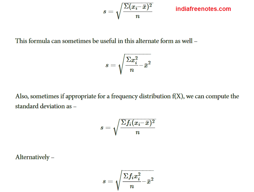
Therefore, we define the formula for the standard deviation of the distribution of a variable X with n data points as:
Variance

Another statistical term that is related to the distribution is the variance, which is the standard deviation squared (variance = SD² ). The SD may be either positive or negative in value because it is calculated as a square root, which can be either positive or negative. By squaring the SD, the problem of signs is eliminated. One common application of the variance is its use in the F-test to compare the variance of two methods and determine whether there is a statistically significant difference in the imprecision between the methods.

In many applications, however, the SD is often preferred because it is expressed in the same concentration units as the data. Using the SD, it is possible to predict the range of control values that should be observed if the method remains stable. As discussed in an earlier lesson, laboratorians often use the SD to impose “gates” on the expected normal distribution of control values.

Coefficient of Variation

Another way to describe the variation of a test is calculate the coefficient of variation, or CV. The CV expresses the variation as a percentage of the mean, and is calculated as follows:

CV% = (SD/Xbar)100

In the laboratory, the CV is preferred when the SD increases in proportion to concentration. For example, the data from a replication experiment may show an SD of 4 units at a concentration of 100 units and an SD of 8 units at a concentration of 200 units. The CVs are 4.0% at both levels and the CV is more useful than the SD for describing method performance at concentrations in between. However, not all tests will demonstrate imprecision that is constant in terms of CV. For some tests, the SD may be constant over the analytical range.

The CV also provides a general “feeling” about the performance of a method. CVs of 5% or less generally give us a feeling of good method performance, whereas CVs of 10% and higher sound bad. However, you should look carefully at the mean value before judging a CV. At very low concentrations, the CV may be high and at high concentrations the CV may be low. For example, a bilirubin test with an SD of 0.1 mg/dL at a mean value of 0.5 mg/dL has a CV of 20%, whereas an SD of 1.0 mg/dL at a concentration of 20 mg/dL corresponds to a CV of 5.0%.
Skewness

Skewness is a statistical measure that indicates the degree and direction of asymmetry in a frequency distribution. When data is distributed evenly around the central value, the distribution is said to be symmetrical. However, if one side of the distribution extends farther than the other, the distribution is skewed.

In Business Statistics, skewness helps researchers and managers understand the nature of data distribution, identify trends, and make informed decisions. It is commonly used in the analysis of income, profits, wages, sales, investment returns, and market behavior.

Definition of Skewness

Skewness refers to the extent to which a distribution deviates from symmetry. It measures whether the observations are concentrated more on one side of the distribution than the other.

A distribution may be:

  • Symmetrical
  • Positively Skewed
  • Negatively Skewed

Types of Skewness

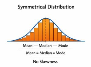
1. Symmetrical Distribution

A symmetrical distribution has equal frequencies on both sides of the central value.

Characteristics

  • Mean = Median = Mode
  • No skewness
  • Skewness coefficient = 0

Example: The distribution of heights of a large group of people often approximates a symmetrical distribution.

Diagram

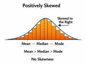
2. Positive Skewness (Right Skewness)

A distribution is positively skewed when the tail extends toward the right side.

Characteristics

  • Mean > Median > Mode
  • More observations are concentrated at lower values.
  • A few high values pull the mean to the right.

Example: Income distribution in many countries where a small number of people earn very high incomes.

Diagram

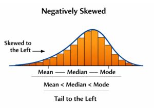
3. Negative Skewness (Left Skewness)

A distribution is negatively skewed when the tail extends toward the left side.

Characteristics

  • Mean < Median < Mode
  • More observations are concentrated at higher values.
  • A few low values pull the mean to the left.

Example: Marks obtained in an easy examination where most students score high marks.

Diagram

Importance of Skewness

  • Helps Understand the Nature of Data Distribution

Skewness helps statisticians and business analysts understand whether a dataset is symmetrical or asymmetrical. It reveals the direction and degree of deviation from a normal distribution. By examining skewness, researchers can identify whether observations are concentrated toward higher or lower values. This understanding is essential for interpreting data accurately. In business statistics, knowing the nature of distribution helps managers evaluate performance, customer behavior, and market trends more effectively, leading to better analysis and decision-making.

  • Assists in Business Decision-Making

Business decisions often depend on accurate interpretation of statistical data. Skewness provides valuable insights into the distribution of sales, profits, costs, and customer preferences. By understanding whether data is positively or negatively skewed, managers can identify unusual patterns and take appropriate actions. It helps in resource allocation, strategic planning, and performance evaluation. Therefore, skewness serves as an important analytical tool that supports informed and rational decision-making in various business activities and organizational operations.

  • Useful in Forecasting and Planning

Forecasting future trends requires a proper understanding of past and present data. Skewness helps identify the distribution pattern of historical observations, enabling analysts to make more accurate predictions. If data is highly skewed, forecasting models may need adjustments to improve reliability. Businesses use skewness while planning production, inventory, marketing strategies, and financial investments. By understanding the direction of data concentration, organizations can anticipate future developments and prepare suitable plans, reducing uncertainty and improving operational efficiency.

  • Helps in Selecting Appropriate Statistical Methods

Many statistical techniques assume that data follows a normal or symmetrical distribution. Skewness helps determine whether these assumptions are valid. If a dataset is highly skewed, analysts may need to use alternative methods or transform the data before analysis. This ensures the accuracy and validity of statistical results. In research and business studies, selecting the correct analytical technique is crucial for drawing reliable conclusions. Therefore, skewness plays an important role in choosing suitable statistical tools and procedures.

  • Identifies the Presence of Extreme Values

Skewness helps detect the influence of extreme values or outliers in a dataset. A highly skewed distribution often indicates that a few observations are significantly larger or smaller than the majority. Identifying such values is important because they can affect averages, forecasts, and business decisions. Managers and researchers can investigate these unusual observations to determine whether they represent genuine trends or data errors. Thus, skewness contributes to more accurate data interpretation and enhances the quality of statistical analysis.

  • Useful in Financial and Investment Analysis

In finance, skewness is widely used to analyze investment returns, stock prices, and financial risks. Investors prefer to understand whether returns are concentrated around gains or losses. Positive and negative skewness provide information about potential opportunities and risks associated with investments. Financial analysts use skewness to evaluate portfolio performance and make informed investment decisions. Therefore, skewness is an important measure in risk assessment, helping businesses and investors manage uncertainty and improve financial planning.

  • Facilitates Comparison of Different Distributions

Skewness enables comparison between different datasets by showing the direction and degree of asymmetry. Two datasets may have similar averages but differ significantly in their distribution patterns. By measuring skewness, analysts can identify these differences and gain deeper insights into the data. Businesses often compare sales performance, customer behavior, employee productivity, and financial results using skewness measures. This comparative analysis helps managers understand relative performance and make more effective decisions based on statistical evidence.

  • Enhances Research and Market Analysis

Skewness is an important tool in research and market analysis because it provides information about consumer behavior, market demand, and economic conditions. Researchers use skewness to study patterns and identify trends within datasets. In marketing, understanding skewed distributions helps businesses segment customers and develop targeted strategies. It also assists in evaluating survey results and market responses. By offering a clearer picture of data behavior, skewness improves the quality of research findings and supports better business and policy decisions.

Limitations of Skewness

  • Highly Sensitive to Extreme Values

One of the major limitations of skewness is its sensitivity to extreme values or outliers. A few unusually large or small observations can significantly influence the skewness coefficient and create a misleading impression of the distribution. In business data, unusual sales figures, profits, or losses may distort the measure of skewness. As a result, the calculated value may not accurately represent the majority of observations. Therefore, analysts must carefully examine the presence of outliers before interpreting skewness and drawing conclusions from statistical data.

  • Does Not Measure Dispersion

Skewness measures only the asymmetry of a distribution and provides no information about the spread or variability of data. Two datasets may have the same skewness value but differ greatly in their dispersion. To understand the complete nature of a distribution, skewness must be used along with measures such as range, variance, and standard deviation. Relying solely on skewness can lead to incomplete analysis. Therefore, it should be considered as one aspect of statistical description rather than a comprehensive measure of data characteristics.

  • Different Methods May Give Different Results

There are several methods of measuring skewness, including Karl Pearson’s, Bowley’s, and Kelly’s coefficients. These methods are based on different statistical concepts and may produce different values for the same dataset. Such variations can create confusion in interpretation and comparison. Analysts may find it difficult to determine which measure best represents the distribution. Consequently, the existence of multiple methods reduces the uniformity of skewness measurement and sometimes complicates statistical analysis, especially when comparing results from different studies or datasets.

  • Difficult to Interpret Precisely

Although skewness indicates the direction and degree of asymmetry, its exact interpretation is often difficult. A positive or negative value shows the direction of skewness, but understanding the practical significance of a particular value may not be straightforward. For example, determining whether a skewness coefficient indicates moderate or severe asymmetry requires additional judgment. This complexity may create challenges for managers, researchers, and students. Therefore, skewness values should be interpreted carefully and in conjunction with graphical analysis and other statistical measures.

  • Not Reliable for Small Samples

Skewness may not provide reliable results when calculated from small samples. In small datasets, a few observations can greatly influence the measure, making it unstable and less representative of the population. Sampling fluctuations may cause skewness values to vary considerably from one sample to another. As a result, conclusions based on skewness from limited data may be misleading. For accurate interpretation, larger datasets are generally preferred. Therefore, analysts should exercise caution when using skewness to evaluate distributions based on small samples.

  • Cannot Fully Describe Distribution Shape

Skewness provides information only about asymmetry and does not fully describe the shape of a distribution. Other characteristics, such as kurtosis, modality, and dispersion, are also important for understanding data behavior. Two distributions may have identical skewness values but differ significantly in other aspects. Consequently, skewness alone cannot provide a complete picture of the dataset. Analysts must combine it with additional statistical measures and graphical tools to gain a thorough understanding of the distribution and make informed decisions.

  • Requires Accurate Data

The accuracy of skewness depends heavily on the quality of the data used. Errors in data collection, recording, classification, or tabulation can affect the calculated skewness coefficient and lead to incorrect conclusions. In business statistics, inaccurate sales, profit, or customer data may distort the measure of asymmetry. Therefore, reliable and properly verified data is essential for meaningful skewness analysis. This dependence on data accuracy represents a limitation because errors at any stage of data handling can reduce the usefulness of skewness measurements.

  • Limited Use When Used Alone

Skewness has limited usefulness when considered in isolation. While it provides information about asymmetry, it does not explain other important characteristics of the dataset. Effective statistical analysis requires the use of multiple measures, including averages, dispersion, and correlation. If skewness is used alone, analysts may overlook critical aspects of data behavior. Therefore, it should be regarded as a supplementary measure rather than a complete analytical tool. Combining skewness with other statistical techniques leads to more accurate interpretations and better decision-making.

Kurtosis

Kurtosis is a statistical measure that describes the degree of peakedness or flatness of a frequency distribution in comparison with a normal distribution. It indicates how observations are concentrated around the mean and how the tails of the distribution behave.

In Business Statistics, kurtosis helps analysts understand the shape of a distribution and identify whether data contains extreme observations. It is widely used in finance, economics, market research, quality control, and risk analysis.

Definition of Kurtosis

Kurtosis is the measure of the shape of a distribution that indicates the extent to which observations cluster around the center and the thickness of the tails relative to a normal distribution.

The term Kurtosis was introduced by Karl Pearson.

Excess Kurtosis

An excess kurtosis is a metric that compares the kurtosis of a distribution against the kurtosis of a normal distribution. The kurtosis of a normal distribution equals 3. Therefore, the excess kurtosis is found using the formula below:

Excess Kurtosis = Kurtosis – 3

Types of Kurtosis

The types of kurtosis are determined by the excess kurtosis of a particular distribution. The excess kurtosis can take positive or negative values as well, as values close to zero.

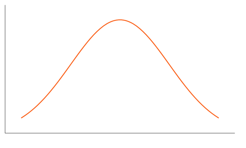
1. Mesokurtic

Mesokurtic Distribution is a distribution that has the same degree of peakedness and tail thickness as a normal distribution. It serves as the standard or benchmark against which other types of kurtosis are compared. In a mesokurtic distribution, observations are moderately concentrated around the mean, and the tails are neither too heavy nor too light. The coefficient of kurtosis (β₂) is equal to 3, while excess kurtosis is 0. Many natural and social phenomena approximately follow a mesokurtic pattern. This type of distribution indicates a balanced spread of data without an unusual concentration of extreme values. In business statistics, mesokurtic distributions are often considered ideal because they reflect a normal and predictable pattern of observations.

Example: The distribution of examination scores in a large class often approximates a mesokurtic distribution.

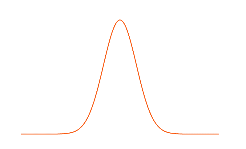
2. Leptokurtic

Leptokurtic Distribution is more peaked than a normal distribution and has heavier tails. In this type of distribution, a large number of observations are concentrated near the mean, while the tails contain more extreme values than a normal distribution. The coefficient of kurtosis (β₂) is greater than 3, and excess kurtosis is positive. Because of its heavy tails, a leptokurtic distribution indicates a higher probability of extreme observations occurring. This characteristic is particularly important in finance and investment analysis, where sudden gains or losses may occur. In business statistics, leptokurtic distributions are useful for identifying situations involving high risk and volatility. The presence of a sharp peak and heavy tails suggests that observations cluster around the center but occasionally produce significant deviations from the average.

Example: Stock market returns often follow a leptokurtic distribution because extreme gains and losses occur more frequently than expected under a normal distribution.

3. Platykurtic

Platykurtic Distribution is flatter than a normal distribution and has lighter tails. In this type of distribution, observations are more evenly spread across the range of data, resulting in a broad and low central peak. The coefficient of kurtosis (β₂) is less than 3, while excess kurtosis is negative. Because the tails are lighter, extreme observations occur less frequently than in a normal distribution. A platykurtic distribution indicates greater dispersion and lower concentration of observations around the mean. In business statistics, such distributions may occur when data is uniformly distributed across different categories. The flatter shape suggests that observations are widely dispersed and that the likelihood of unusually high or low values is relatively small.

Example: The distribution of customer arrivals spread evenly throughout a day may exhibit a platykurtic pattern.

Karl Pearson and Spearman Rank Correlation

Karl Pearson Coefficient of Correlation

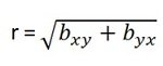
Karl Pearson Coefficient of Correlation (also called the Pearson correlation coefficient or Pearson’s r) is a measure of the strength and direction of the linear relationship between two variables. It ranges from -1 to +1, where +1 indicates a perfect positive linear relationship, -1 indicates a perfect negative linear relationship, and 0 indicates no linear relationship. The formula for Pearson’s r is calculated by dividing the covariance of the two variables by the product of their standard deviations. It is widely used in statistics to analyze the degree of correlation between paired data.

The following are the main properties of correlation.

1. Coefficient of Correlation lies between -1 and +1:

The coefficient of correlation cannot take value less than -1 or more than one +1. Symbolically,

-1<=r<= + 1 or | r | <1.

2. Coefficients of Correlation are independent of Change of Origin:

This property reveals that if we subtract any constant from all the values of X and Y, it will not affect the coefficient of correlation.

3. Coefficients of Correlation possess the property of symmetry:

The degree of relationship between two variables is symmetric as shown below:

4. Coefficient of Correlation is independent of Change of Scale:

This property reveals that if we divide or multiply all the values of X and Y, it will not affect the coefficient of correlation.

5. Co-efficient of correlation measures only linear correlation between X and Y.

6. If two variables X and Y are independent, coefficient of correlation between them will be zero.

Karl Pearson’s Coefficient of Correlation is widely used mathematical method wherein the numerical expression is used to calculate the degree and direction of the relationship between linear related variables.

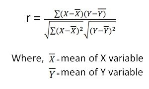
Pearson’s method, popularly known as a Pearsonian Coefficient of Correlation, is the most extensively used quantitative methods in practice. The coefficient of correlation is denoted by “r”.

If the relationship between two variables X and Y is to be ascertained, then the following formula is used:

Properties of Coefficient of Correlation

  • The value of the coefficient of correlation (r) always lies between±1. Such as:r = +1, perfect positive correlation

    r = -1, perfect negative correlation

    r = 0, no correlation

  • The coefficient of correlation is independent of the origin and scale.By origin, it means subtracting any non-zero constant from the given value of X and Y the vale of “r” remains unchanged. By scale it means, there is no effect on the value of “r” if the value of X and Y is divided or multiplied by any constant.
  • The coefficient of correlation is a geometric mean of two regression coefficient. Symbolically it is represented as:
  • The coefficient of correlation is “ zero” when the variables X and Y are independent. But, however, the converse is not true.

Assumptions of Karl Pearson’s Coefficient of Correlation

  • The relationship between the variables is “Linear”, which means when the two variables are plotted, a straight line is formed by the points plotted.
  • There are a large number of independent causes that affect the variables under study so as to form a Normal Distribution. Such as, variables like price, demand, supply, etc. are affected by such factors that the normal distribution is formed.
  • The variables are independent of each other.                                     

Note: The coefficient of correlation measures not only the magnitude of correlation but also tells the direction. Such as, r = -0.67, which shows correlation is negative because the sign is “-“ and the magnitude is 0.67.

Spearman Rank Correlation

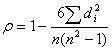
Spearman rank correlation is a non-parametric test that is used to measure the degree of association between two variables.  The Spearman rank correlation test does not carry any assumptions about the distribution of the data and is the appropriate correlation analysis when the variables are measured on a scale that is at least ordinal.

The Spearman correlation between two variables is equal to the Pearson correlation between the rank values of those two variables; while Pearson’s correlation assesses linear relationships, Spearman’s correlation assesses monotonic relationships (whether linear or not). If there are no repeated data values, a perfect Spearman correlation of +1 or −1 occurs when each of the variables is a perfect monotone function of the other.

Intuitively, the Spearman correlation between two variables will be high when observations have a similar (or identical for a correlation of 1) rank (i.e. relative position label of the observations within the variable: 1st, 2nd, 3rd, etc.) between the two variables, and low when observations have a dissimilar (or fully opposed for a correlation of −1) rank between the two variables.

The following formula is used to calculate the Spearman rank correlation:

ρ = Spearman rank correlation

di = the difference between the ranks of corresponding variables

n = number of observations

Assumptions

The assumptions of the Spearman correlation are that data must be at least ordinal and the scores on one variable must be monotonically related to the other variable.

Least Square Method

The least square method is the process of finding the best-fitting curve or line of best fit for a set of data points by reducing the sum of the squares of the offsets (residual part) of the points from the curve. During the process of finding the relation between two variables, the trend of outcomes are estimated quantitatively. This process is termed as regression analysis. The method of curve fitting is an approach to regression analysis. This method of fitting equations which approximates the curves to given raw data is the least square.

It is quite obvious that the fitting of curves for a particular data set are not always unique. Thus, it is required to find a curve having a minimal deviation from all the measured data points. This is known as the best-fitting curve and is found by using the least-squares method.

Least Square Method

The least-squares method is a crucial statistical method that is practised to find a regression line or a best-fit line for the given pattern. This method is described by an equation with specific parameters. The method of least squares is generously used in evaluation and regression. In regression analysis, this method is said to be a standard approach for the approximation of sets of equations having more equations than the number of unknowns.

The method of least squares actually defines the solution for the minimization of the sum of squares of deviations or the errors in the result of each equation. Find the formula for sum of squares of errors, which help to find the variation in observed data.

The least-squares method is often applied in data fitting. The best fit result is assumed to reduce the sum of squared errors or residuals which are stated to be the differences between the observed or experimental value and corresponding fitted value given in the model.

There are two basic categories of least-squares problems:

  • Ordinary or linear least squares
  • Nonlinear least squares

These depend upon linearity or nonlinearity of the residuals. The linear problems are often seen in regression analysis in statistics. On the other hand, the non-linear problems generally used in the iterative method of refinement in which the model is approximated to the linear one with each iteration.

Least Square Method Graph

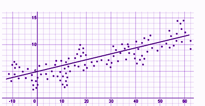
In linear regression, the line of best fit is a straight line as shown in the following diagram:

The given data points are to be minimized by the method of reducing residuals or offsets of each point from the line. The vertical offsets are generally used in surface, polynomial and hyperplane problems, while perpendicular offsets are utilized in common practice.

Least Square Method Formula

The least-square method states that the curve that best fits a given set of observations, is said to be a curve having a minimum sum of the squared residuals (or deviations or errors) from the given data points. Let us assume that the given points of data are (x1,y1), (x2,y2), (x3,y3), …, (xn,yn) in which all x’s are independent variables, while all y’s are dependent ones. Also, suppose that f(x) be the fitting curve and d represents error or deviation from each given point.

Now, we can write:

d1 = y1 − f(x1)

d2 = y2 − f(x2)

d3 = y3 − f(x3)

…..

dn = yn – f(xn)

The least-squares explain that the curve that best fits is represented by the property that the sum of squares of all the deviations from given values must be minimum. i.e:

Sum = Minimum Quantity

Limitations for Least-Square Method

The least-squares method is a very beneficial method of curve fitting. Despite many benefits, it has a few shortcomings too. One of the main limitations is discussed here.

In the process of regression analysis, which utilizes the least-square method for curve fitting, it is inevitably assumed that the errors in the independent variable are negligible or zero. In such cases, when independent variable errors are non-negligible, the models are subjected to measurement errors. Therefore, here, the least square method may even lead to hypothesis testing, where parameter estimates and confidence intervals are taken into consideration due to the presence of errors occurring in the independent variables.

Secondary Data: Merits, Limitations, Sources

Secondary data is the data that have been already collected by and readily available from other sources. Such data are cheaper and more quickly obtainable than the primary data and also may be available when primary data can not be obtained at all.

Advantages of Secondary data

  1. It is economical. It saves efforts and expenses.
  2. It is time saving.
  3. It helps to make primary data collection more specific since with the help of secondary data, we are able to make out what are the gaps and deficiencies and what additional information needs to be collected.
  4. It helps to improve the understanding of the problem.
  5. It provides a basis for comparison for the data that is collected by the researcher.

Disadvantages of Secondary Data

  1. Secondary data is something that seldom fits in the framework of the marketing research factors. Reasons for its non-fitting are:
  • Unit of secondary data collection: Suppose you want information on disposable income, but the data is available on gross income. The information may not be same as we require.
  • Class Boundaries may be different when units are same.
Before 5 Years After 5 Years
2500-5000 5000-6000
5001-7500 6001-7000
7500-10000 7001-10000
  1. Thus the data collected earlier is of no use to you.
  1. Accuracy of secondary data is not known.
  2. Data may be outdated.

Evaluation of Secondary Data

Because of the above mentioned disadvantages of secondary data, we will lead to evaluation of secondary data. Evaluation means the following four requirements must be satisfied:

  1. Availability: It has to be seen that the kind of data you want is available or not. If it is not available then you have to go for primary data.
  2. Relevance: It should be meeting the requirements of the problem. For this we have two criteria:
    1. Units of measurement should be the same.
    2. Concepts used must be same and currency of data should not be outdated.
  3. Accuracy: In order to find how accurate, the data is, the following points must be considered: –
  • Specification and methodology used
  • Margin of error should be examined
  • The dependability of the source must be seen.

4. Sufficiency: Adequate data should be available.

Robert W Joselyn has classified the above discussion into eight steps. These eight steps are sub classified into three categories. He has given a detailed procedure for evaluating secondary data.

  • Applicability of research objective.
  • Cost of acquisition.
  • Accuracy of data.

Data: Relevance of data in Current scenario

This data comes from everywhere: sensors used to gather climate information, posts to social media sites, digital pictures and videos, purchase transaction records, and cell phone GPS signals to name a few. This data is big data. What has also changed in the last decade is that we now have the means to sift through these 2.5 quintillion bytes of data in a reasonable amount of time. All these changes have major implications for organizations today.

In organizations, analytics enables professionals to convert extensive data and statistical and quantitative analysis into powerful insights that can drive efficient decisions.

Therefore with analytics, organizations can now base their decisions and strategies on data rather than on gut feelings. Moreover, with the rate at which this data can be analyzed, organizations are able to keep tabs on the customer trends in near real time. As a result effectiveness of a strategy can be determined almost immediately. Thus with powerful insights, analytics promises reduced costs and increased profits.
The analytics Industry is one of the fastest growing in modern times with it poised to become a $50 billion market by 2017. With this sudden surge in the analytics industry, there is a tremendous increase in the demand for analytics expertise across all domains, throughout all major organizations across the globe. It has been predicted that by 2018, the United States alone could face a shortage of 140,000 to 190,000 people with deep analytical skills as well as 1.5 million managers and analysts with the know-how to use the analysis of big data to make effective decisions.
IBM’s recent study revealed that “83% of Business Leaders listed Business Analytics as the top priority in their business priority list.”
Deloitte has mentioned in its study that: Decision makers who can leverage everyday data & information into actionable insights for the growth of their organization by taking reliable decisions, will find themselves in a much better position to achieve strategic growth in their career.

There is an information overload in today’s world and data analytics helps to cut out the clutter to help businesses make safe and smart choices.

A recent report by Nucleus Research found that companies realize a return of USD10.66 for every dollar they invest in analytics.

In the developed economies of Europe, government administrators could save more than €100 billion ($149 billion) in operational efficiency improvements alone by using big data, not including using big data to reduce fraud and errors and boost the collection of tax revenues. Thus big data courses in India are going to be essential in a few years.

There is a saying “Today Data is the new Oil”. Data in today’s business & technology world is absolutely crucial. The Big Data technologies and initiatives are rising to analyze this data for gaining insights that can help in making strategic decisions. The concept evolved at the beginning of 21st century, and every technology giant is now making use of Big Data technologies. Big Data refers to vast data sets that may be structured or unstructured. There is a massive amount of data which has been produced everyday by businesses & users alike. Big data analytics is the process of examining large data sets to find the underlying insights & patterns. Data analytics field is absolutely vast.

The Big Data Analytics is indeed a revolution in the field of information technology. The use of Data analytics by the companies is increasing day by day. The primary focus of the companies is on the customers. Hence this field is flourishing in the area of B2C applications. There are 3 divisions of Big data analytics: Prescriptive Analytics, Predictive Analytics, Descriptive Analytics. There are four different perspectives to explain why big data analytics is so important. They are

  • Data Science Perspective
  • Business Perspective
  •  Real Time Usability Perspective
  • Job Market Perspective

Big Data Analytics & Data Science

The analytics involves the use of advanced techniques & tools of analytics on a data obtained via different sources & different sizes. Big Data has the properties of high variety, volume & velocity. The data sets are basically retrieved from various online networks, web pages, audio & video devices, social media, logs & many other sources.

It involves the use of techniques like machine learning, data mining, natural language processing & statistics. The data is extracted, prepared & blended to provide analysis for the businesses.

Benefits of Big Data Analytics

Due to enormous growth in the field of Big Data Analytics it is extensively used in multiple industries like

  • Banking
  • Healthcare
  • Energy
  • Technology
  • Consumer
  • Manufacturing

The importance of big data analytics leads to intense competition and increased demand for big data professionals. Data Science and Analytics is an evolving field with huge potential. Data analytics help in analyzing the value chain of business and gain insights. The use of analytics can enhance the industry knowledge of the analysts. Data analytics experts provide the organizations a chance to learn about the opportunities for the business.

Types of Date: Primary & Secondary

Primary data

Primary data are original observations collected by the researcher or his agent for the first time for any investigation and used by them in the statistical analysis.

The primary data is the one type of important data. It is collection of data from first-hand information.

This information published by one organization for some purposes. This type of primary data is mostly pure and original data.

The primary data collection is having three different data collection methods are:

  • Data Collection through Investigation:

In this method, trained investigators are working as employees for collecting the data. The researchers will use the tools like interview and collect the information from the individual persons.

  • Personal Investigation Methods:

The researchers or the data collectors will conduct the survey and hence they collect the data. In this method we have to collect more accurate data and original data. This method is useful for small data collection only not big collection of data projects.

  • Data Collection through Telephones:

The data researcher uses the tools like telephones, mobile phones to collect the information or data. This is accurate and very quick process for data collection. But information collected is not accurate and true.

(2) secondary data

The secondary data is the other type of data, which is collection of data from second hand information. This information is known as, given data is already collected from any one person for some purpose, and it has available for the present issues. And mostly these secondary data are not relevant and pure or original data.

Primary Data Census vs Samples

In Statistics, the basis of all statistical calculations or interpretation lies in the collection of data. There are numerous methods of data collection. In this lesson, we shall focus on two primary methods and understand the difference between them. Both are suitable in different cases and the knowledge of these methods is important to understand when to apply which method. These two methods are the Census method and Sampling method.

Census Method

Census method is the method of statistical enumeration where all members of the population are studied. A population refers to the set of all observations under concern. For example, if you want to carry out a survey to find out student’s feedback about the facilities of your school, all the students of your school would form a part of the ‘population’ for your study.

At a more realistic level, a country wants to maintain information and records about all households. It can collect this information by surveying all households in the country using the census method.

In our country, the Government conducts the Census of India every ten years. The Census appropriates information from households regarding their incomes, the earning members, the total number of children, members of the family, etc. This method must take into account all the units. It cannot leave out anyone in collecting data. Once collected, the Census of India reveals demographic information such as birth rates, death rates, total population, population growth rate of our country, etc. The last census was conducted in the year 2011.

Sampling Method

Like we have studied, the population contains units with some similar characteristics on the basis of which they are grouped together for the study. In the case of the Census of India, for example, the common characteristic was that all units are Indian nationals. But it is not always practical to collect information from all the units of the population.

It is a time-consuming and costly method. Thus, an easy way out would be to collect information from some representative group from the population and then make observations accordingly. This representative group which contains some units from the whole population is called the sample.

The first most important step in selecting a sample is to determine the population. Once the population is identified, a sample must be selected. A good sample is one which is:

  • Small in size.
  • It provides adequate information about the whole population.
  • It takes less time to collect and is less costly.

In the case of our previous example, you could choose students from your class to be the representative sample out of the population (all students in the school). However, there must be some rationale behind choosing the sample. If you think your class comprises a set of students who will give unbiased opinions/feedback or if you think your class contains students from different backgrounds and their responses would be relevant to your student, you must choose them as your sample. Otherwise, it is ideal to choose another sample which might be more relevant.

Again, realistically, the government wants estimates on the average income of the Indian household. It is difficult and time-consuming to study all households. The government can simply choose, say, 50 households from each state of the country and calculate the average of that to arrive at an estimate. This estimate is not necessarily the actual figure that would be arrived at if all units of the population underwent study. But it approximately gives an idea of what the figure might look like.

Difference between Census and Sample Surveys

Parameter

Census

Sample Survey

Definition A statistical method that studies all the units or members of a population. A statistical method that studies only a representative group of the population, and not all its members.
Calculation Total/Complete Partial
Time involved It is a time-consuming process. It is a quicker process.
Cost involved It is a costly method. It is a relatively inexpensive method.
Accuracy The results obtained are accurate as each member is surveyed. So, there is a negligible error. The results are relatively inaccurate due to leaving out of items from the sample. The resulting error is large.
Reliability Highly reliable Low reliability
Error Not present The smaller the sample size, the larger the error.
Relevance This method is suited for heterogeneous data. This method is suited for homogeneous data.

Methods of Primary Data Collection: Observation, Interview, Questionnaire, and Survey

Primary Data is information collected firsthand by a researcher for a specific research purpose. It is original, fresh, and tailored directly to the research question or objective. Methods such as surveys, interviews, experiments, and observations are commonly used to gather primary data. Since it is collected directly from the source, primary data is highly relevant, specific, and accurate. However, it often requires more time, effort, and resources compared to using existing information. It is essential for studies needing updated or detailed insights.

Methods of Primary Data Collection:

  • Observation

Observation involves systematically watching and recording behaviors, events, or phenomena as they occur naturally or in a controlled setting. It allows researchers to gather real-time, unbiased data without influencing the subject’s behavior. Observations can be structured (following a predefined checklist) or unstructured (open-ended). It is especially useful when participants are unwilling or unable to provide accurate verbal responses. Researchers may act as participants (participant observation) or as non-intrusive observers. Observation is widely used in fields like anthropology, psychology, and marketing to understand behaviors, workflows, or consumer interactions. It provides deep insights but may sometimes lack the ability to explain the reasons behind certain actions, requiring combination with other methods like interviews for richer analysis.

  • Interview

An interview is a direct, face-to-face, telephonic, or video-based conversation between the researcher and the participant aimed at gathering detailed information. Interviews can be structured (fixed questions), semi-structured (guided by a framework but flexible), or unstructured (open conversation). This method allows for in-depth exploration of opinions, emotions, experiences, and motivations. Interviews can be personal or group-based, depending on research needs. They are commonly used in qualitative research to gain comprehensive understanding and context behind responses. Although interviews provide rich, detailed data, they can be time-consuming and may introduce biases if not conducted carefully. Proper interviewer skills are essential for encouraging honest and open communication from participants.

  • Questionnaire

Questionnaire is a set of written or digital questions designed to collect information from respondents. It can include closed-ended questions (like multiple-choice) or open-ended questions (where respondents write answers in their own words). Questionnaires are often used for surveys and research studies where standardized information is needed from a large audience. They are cost-effective, easy to distribute, and efficient in data collection. Responses are easy to quantify for statistical analysis. However, the design of the questionnaire is crucial — poorly framed questions can lead to misunderstandings and unreliable data. Questionnaires are widely used in education, social science, market research, and customer satisfaction studies.

  • Survey

Survey is a research method involving the systematic collection of information from a sample of individuals, usually through questionnaires or interviews. Surveys can be conducted in-person, via phone, online, or by mail. They are useful for gathering quantitative as well as qualitative data about behaviors, attitudes, preferences, or demographics. Surveys are popular because they can cover large populations at relatively low cost and produce statistically significant results if designed properly. However, their effectiveness depends on clear question framing, respondent honesty, and sampling methods. Surveys are widely used in fields like business, healthcare, political science, and social research for decision-making and trend analysis.

error: Content is protected !!