Determination of Season

Time series datasets can contain a seasonal component.

This is a cycle that repeats over time, such as monthly or yearly. This repeating cycle may obscure the signal that we wish to model when forecasting, and in turn may provide a strong signal to our predictive models.

  • The definition of seasonality in time series and the opportunity it provides for forecasting with machine learning methods.
  • How to use the difference method to create a seasonally adjusted time series of daily temperature data.
  • How to model the seasonal component directly and explicitly subtract it from observations.

Seasonality in Time Series

Time series data may contain seasonal variation.

Seasonal variation, or seasonality, are cycles that repeat regularly over time.

A repeating pattern within each year is known as seasonal variation, although the term is applied more generally to repeating patterns within any fixed period.

Introductory Time Series with R

A cycle structure in a time series may or may not be seasonal. If it consistently repeats at the same frequency, it is seasonal, otherwise it is not seasonal and is called a cycle.

Benefits to Machine Learning

Understanding the seasonal component in time series can improve the performance of modeling with machine learning.

This can happen in two main ways:

  • Clearer Signal: Identifying and removing the seasonal component from the time series can result in a clearer relationship between input and output variables.
  • More Information: Additional information about the seasonal component of the time series can provide new information to improve model performance.

Both approaches may be useful on a project. Modeling seasonality and removing it from the time series may occur during data cleaning and preparation.

Extracting seasonal information and providing it as input features, either directly or in summary form, may occur during feature extraction and feature engineering activities.

Types of Seasonality

There are many types of seasonality; for example:

  • Time of Day.
  • Daily.
  • Weekly.
  • Monthly.
  • Yearly.

As such, identifying whether there is a seasonality component in your time series problem is subjective.

The simplest approach to determining if there is an aspect of seasonality is to plot and review your data, perhaps at different scales and with the addition of trend lines.

Removing Seasonality

Once seasonality is identified, it can be modeled.

The model of seasonality can be removed from the time series. This process is called Seasonal Adjustment, or Deseasonalizing.

A time series where the seasonal component has been removed is called seasonal stationary. A time series with a clear seasonal component is referred to as non-stationary.

There are sophisticated methods to study and extract seasonality from time series in the field of Time Series Analysis. As we are primarily interested in predictive modeling and time series forecasting, we are limited to methods that can be developed on historical data and available when making predictions on new data.

In this tutorial, we will look at two methods for making seasonal adjustments on a classical meteorological-type problem of daily temperatures with a strong additive seasonal component. Next, let’s take a look at the dataset we will use in this tutorial.

Index Number, Meaning, Definition, Features, Types, Steps, Components, Applications, Advantages and Limitations

Index Number is a statistical tool used to measure changes in economic variables over time, such as prices, quantities, or values. It expresses the relative change of a variable compared to a base period, usually set at 100. Index numbers help compare data across time, eliminating the effects of units or scales. They are widely used in economics and business to track inflation (e.g., Consumer Price Index), production, or cost changes. There are different types, including price index, quantity index, and value index. Methods of calculation include Laspeyres’, Paasche’s, and Fisher’s index. Index numbers simplify complex data, supporting decision-making and policy formulation in business and government.

Definition of Index Number

An Index Number is a statistical device that measures the relative change in the level of a phenomenon with respect to a base period, which is generally taken as 100.

Example of an Index Number

Suppose the price of a product was ₹50 in the base year and ₹75 in the current year.

Price Index = (75 / 50) × 100

This indicates that the price has increased by 50% compared to the base year.

Features of Index Numbers

  • Statistical Device for Comparison

Index numbers serve as a powerful statistical tool to measure and compare relative changes in variables over time or location. They reduce complex and bulky data into a single, easily understandable figure. By converting raw data into percentage form based on a base year, they help highlight changes and trends in variables like prices, output, wages, etc. For instance, comparing consumer prices in different years becomes simpler and more effective using a price index. This comparative capability makes index numbers essential in economic and business decision-making.

  • Measure of Relative Change

Index numbers are primarily designed to show the relative change rather than absolute change. They express how much a variable has increased or decreased in percentage terms compared to a base period. For example, if a price index for a commodity is 125, it means there has been a 25% increase from the base year. This ability to convey relative movement enables users to quickly grasp the extent and direction of change, making index numbers a practical instrument for analyzing economic and financial performance.

  • Base Year Reference

Every index number uses a base year, which serves as the point of comparison. The value for the base year is always taken as 100, and all other values are expressed relative to it. Choosing an appropriate and normal base year is crucial, as it affects the accuracy and interpretation of the index. A well-chosen base year ensures that the index truly reflects meaningful changes over time. Without a base year, the concept of measuring “change” becomes invalid, as comparison needs a consistent starting point.

  • Simplifies Complex Data

Index numbers simplify the analysis of large datasets by converting varied data into a single number. Instead of tracking multiple prices or quantities individually, an index number consolidates the information into one comparable figure. This feature is especially useful in fields like economics, where analyzing movements in prices, costs, or production across different goods and services would otherwise be cumbersome. By providing a summarized measure, index numbers allow business managers, economists, and policymakers to quickly assess trends and make informed decisions.

  • Helps in Economic Analysis and Policy Making

Index numbers are essential tools in economic analysis and government policy formulation. They help track inflation, cost of living, industrial production, and other macroeconomic indicators. For example, the Consumer Price Index (CPI) is often used to adjust salaries and pensions to keep pace with inflation. Index numbers also guide central banks in framing monetary policy. By showing the direction and intensity of economic changes, they provide a factual basis for interventions, budgeting, and strategic planning, ensuring decisions are data-driven and aligned with current economic trends.

  • Various Types for Different Purposes

There are different kinds of index numbers, such as price index, quantity index, and value index, each serving specific needs. A Price Index tracks changes in the price level of goods and services, a Quantity Index measures changes in the physical quantity of goods, and a Value Index reflects changes in total monetary value. This classification makes index numbers versatile for business and economic use. Depending on the objective, businesses can choose the right type to measure trends in cost, output, or revenue over time.

Types of Index Numbers

Index Numbers are classified according to the purpose for which they are constructed. They measure changes in prices, quantities, values, cost of living, production, and other economic activities over time. The main types of index numbers are explained below.

1. Price Index Number

Price Index Number measures changes in the prices of goods and services over a period of time. It shows whether prices have increased or decreased compared to the base period. Price indices are widely used to measure inflation and changes in purchasing power.

Example: If the price index rises from 100 to 120, it indicates a 20% increase in the general price level.

Uses

  • Measuring inflation.
  • Formulating pricing policies.
  • Economic analysis.

2. Quantity Index Number

Quantity Index Number measures changes in the quantity of goods produced, sold, consumed, or transported over time. It helps determine whether the volume of economic activity has increased or decreased.

Example: An index measuring the annual production of automobiles in a country.

Uses

  • Production analysis.
  • Demand assessment.
  • Economic growth measurement.

3. Value Index Number

Value Index Number measures changes in the total monetary value of goods and services. It reflects the combined effect of changes in both prices and quantities.

Formula: Value Index = (Current Year Value / Base Year Value) × 100

Uses

  • Sales analysis.
  • Revenue comparison.
  • Business performance evaluation.

4. Cost of Living Index Number

Cost of Living Index Number measures changes in the cost of maintaining a particular standard of living. It indicates how much consumers need to spend to purchase a fixed basket of goods and services.

Example: Consumer Price Index (CPI).

Uses

  • Wage adjustments.
  • Salary revisions.
  • Inflation measurement.

5. Consumer Price Index (CPI)

Consumer Price Index measures changes in the retail prices of goods and services commonly purchased by consumers. It is one of the most widely used measures of inflation.

Example: The CPI tracks changes in food, housing, transportation, and healthcare costs.

Uses

  • Measuring inflation.
  • Determining dearness allowance.
  • Economic policy formulation.

6. Wholesale Price Index (WPI)

Wholesale Price Index measures changes in the prices of goods at the wholesale level before they reach consumers. It reflects price movements in bulk transactions.

Example: Changes in wholesale prices of agricultural and industrial products.

Uses

  • Monitoring inflation trends.
  • Economic planning.
  • Business pricing decisions.

7. Industrial Production Index (IPI)

Industrial Production Index measures changes in the output of industries such as manufacturing, mining, and electricity generation.

Example: An index showing annual growth in manufacturing production.

Uses

  • Assessing industrial growth.
  • Economic performance analysis.
  • Policy-making.

8. Employment Index Number

Employment Index Number measures changes in employment levels over time. It indicates whether the number of employed persons is increasing or decreasing.

Example: An index tracking employment growth in the manufacturing sector.

Uses

  • Labor market analysis.
  • Workforce planning.
  • Economic assessment.

9. Agricultural Production Index Number

This index measures changes in agricultural output over time. It reflects growth or decline in the production of crops and agricultural products.

Example: An index showing annual wheat production trends.

Uses

  • Agricultural planning.
  • Food security assessment.
  • Policy formulation.

10. Stock Market Index Number

Stock Market Index Number measures changes in the prices of selected shares traded in the stock market. It indicates the overall performance of the stock market.

Examples

  • BSE Sensex
  • NIFTY 50

Uses

  • Investment analysis.
  • Market performance evaluation.
  • Economic forecasting.

Steps in the Construction of Price Index Numbers

Step 1. Define the Purpose and Scope

The first step is to clearly define the objective of the price index—whether it is to measure inflation, cost of living, wholesale prices, or retail prices. This helps determine the type of price index required. The scope includes deciding whether the index will cover all goods and services or only selected ones. A well-defined purpose ensures relevance, consistency, and applicability of the index in real-world decision-making. It also helps identify the target population or sector to which the index will apply.

Step 2. Selection of the Base Year

A base year is the benchmark period against which changes in prices are measured. It is assigned an index value of 100. The base year should be a normal year, free from major economic fluctuations such as inflation, deflation, war, or natural disasters. A well-chosen base year ensures that the comparisons made over time are valid and meaningful. The base year must be recent enough to be relevant, yet stable enough to serve as a reliable point of reference for future comparisons.

Step 3. Selection of Commodities

The selection of goods and services included in the index must reflect the consumption habits of the population or sector under study. The commodities should be representative, regularly used, and available in most markets. The number of items should be sufficient to provide accurate results but not too large to make data collection and computation difficult. For example, a Consumer Price Index may include food, clothing, housing, and transportation items that are commonly consumed by the average household.

Step 4. Collection of Prices

Prices of the selected commodities must be collected for both the base year and the current year. The data should be obtained from reliable sources such as retail stores, wholesale markets, government publications, or official agencies. It is essential to ensure uniformity in the quality, quantity, and unit of measurement of the items while collecting prices. The method of price collection (monthly, quarterly, annually) should also be decided in advance. Accurate and consistent price data is crucial for the credibility of the index.

Step 5. Selection of the Weighting System

Weights are assigned to commodities based on their relative importance or share in total consumption. Heavier weights are given to goods with larger expenditure shares. There are two main types of index numbers: unweighted (all items treated equally) and weighted (different weights for different items). Weighted indices provide more accurate results because they reflect real consumption patterns. The weights can be based on expenditure surveys or input-output data. Common weighting methods include Laspeyres, Paasche, and Fisher’s index formulas.

Step 6. Choice of Formula for Index Calculation

Several formulas exist for calculating price index numbers, each with different assumptions and uses. The most common are:

  • Laspeyres’ Index: Uses base year quantities as weights.

  • Paasche’s Index: Uses current year quantities as weights.

  • Fisher’s Index: Geometric mean of Laspeyres and Paasche.

The choice depends on the data available and the intended use of the index. The selected formula must be consistent, logical, and easy to interpret. It should ideally satisfy the tests of a good index number.

Step 7. Computation and Interpretation

Once the data is collected and the formula chosen, the index number is calculated. The resulting figure shows how much prices have increased or decreased relative to the base year. An index above 100 indicates a rise in prices; below 100 indicates a fall. After computation, the index should be analyzed and interpreted in light of the economic conditions. The final index number can then be published or used for policy decisions, wage adjustments, or business strategy formulation.

Components of an Index Number

Index Numbers are constructed using several essential components that ensure accurate measurement and comparison of changes over time. These components form the foundation of index number calculation and interpretation.

1. Base Period

Base Period is the reference period against which all other periods are compared. It is usually assigned an index value of 100. The base period should be a normal period free from unusual economic conditions such as inflation, recession, or natural disasters. All changes in prices, quantities, or values are measured relative to this period. Selecting an appropriate base period is crucial because it directly affects the reliability and usefulness of the index number. A well-chosen base period provides a meaningful basis for comparison and trend analysis.

2. Current Period

Current Period is the period for which the index number is calculated and compared with the base period. It represents the present situation or the period under study. The values of prices, quantities, or other variables in the current period are used to determine the extent of change from the base period. By comparing current data with base-period data, analysts can measure growth, decline, or stability. This component helps businesses and economists understand recent developments and assess current economic or business performance.

3. Items Included in the Index

Items Included refer to the goods, services, or variables selected for constructing the index number. The choice of items depends on the purpose of the index. For example, a consumer price index may include food, clothing, housing, transportation, and healthcare. The selected items should be representative of the phenomenon being measured. Proper selection ensures that the index accurately reflects actual changes. If important items are omitted or irrelevant items are included, the index may produce misleading results and reduce its practical usefulness.

4. Price or Quantity Data

Price or Quantity Data is essential for constructing index numbers. Depending on the type of index, information regarding prices, quantities, or values is collected for both the base period and the current period. Reliable data ensures that the calculated index reflects real changes rather than errors in measurement. Businesses, governments, and researchers often obtain data from surveys, market reports, official statistics, and business records. The quality of the index number depends greatly on the accuracy, consistency, and completeness of the underlying data.

5. Weights

Weights represent the relative importance of different items included in the index. Not all goods or services contribute equally to consumption, production, or economic activity. Therefore, weights are assigned to reflect their significance. For example, food may receive a higher weight than entertainment in a consumer price index because consumers spend more on food. Weighted index numbers provide more realistic and accurate results than unweighted indices. Proper weighting ensures that the index reflects actual economic conditions and consumer behavior more effectively.

6. Price Relatives

Price Relative is the ratio of the current period price to the base period price, usually expressed as a percentage. It indicates how much the price of an item has changed over time.

Formula: Price Relative=  P1 / P0 × 100

Where:

  • P₁ = Current Period Price
  • P₀ = Base Period Price

Price relatives serve as building blocks for many index number calculations. They simplify the comparison of individual items and help measure overall price changes accurately.

7. Method of Calculation

Method of Calculation is another important component of an index number. Different methods may be used depending on the objective and nature of the data. Common methods include the Simple Aggregative Method, Simple Average of Relatives Method, Laspeyres Method, Paasche Method, and Fisher’s Ideal Method. The choice of method influences the final value of the index. Therefore, selecting an appropriate calculation method is essential for obtaining meaningful and reliable results that accurately represent changes in the variable under study.

8. Purpose of the Index

Every index number is constructed for a specific Purpose. The purpose determines the selection of items, data sources, weights, and calculation methods. For example, an inflation index focuses on price changes, while a production index measures changes in output. Clearly defining the purpose ensures that the index serves its intended function effectively. It also helps users interpret the results correctly. Whether used for business planning, policy formulation, wage adjustments, or economic analysis, the purpose guides the entire process of index number construction.

Applications of Index Numbers in Business

  • Measuring Inflation and Price Changes

Index numbers are widely used to measure inflation and changes in the general price level. Businesses monitor price indices such as the Consumer Price Index (CPI) and Wholesale Price Index (WPI) to understand how prices are changing over time. Rising inflation affects production costs, selling prices, and consumer purchasing power. By analyzing these indices, managers can make appropriate pricing and budgeting decisions. This application helps businesses maintain profitability and adapt to changing economic conditions. Therefore, index numbers play a crucial role in tracking inflation and supporting effective business management.

  • Assisting in Pricing Decisions

Businesses use index numbers to formulate pricing strategies. Changes in raw material costs, labor expenses, and market prices can significantly affect product pricing. By studying relevant price indices, organizations can determine whether product prices need adjustment. This helps ensure that selling prices remain competitive while maintaining profit margins. Index-based pricing decisions are particularly useful in industries where costs fluctuate frequently. As a result, businesses can respond quickly to economic changes and maintain stability in their pricing policies.

  • Sales Performance Analysis

Index numbers help businesses evaluate sales performance over different periods. By converting sales figures into index form, managers can compare growth rates and identify trends more easily. Sales indices show whether sales have increased, decreased, or remained stable compared to a base period. This information assists in assessing the effectiveness of marketing campaigns and sales strategies. Through performance analysis, businesses can identify strengths and weaknesses and implement corrective measures to improve future sales results.

  • Demand Forecasting

Businesses use index numbers to analyze market demand and forecast future customer requirements. Demand-related indices provide information about consumption patterns and market trends. By examining these indices, organizations can estimate future demand for products and services. Accurate demand forecasting helps businesses plan production, manage inventory, and allocate resources efficiently. It also reduces the risk of stock shortages or overproduction. Thus, index numbers support better operational planning and enhance overall business performance.

  • Wage and Salary Adjustments

Many organizations use cost-of-living index numbers to revise wages and salaries. Inflation reduces the purchasing power of employees, making periodic adjustments necessary. By referring to cost-of-living indices, businesses can determine appropriate increases in wages, dearness allowances, and employee benefits. This helps maintain employee satisfaction and financial well-being. Wage adjustments based on index numbers also promote fairness and consistency in compensation policies. Consequently, businesses can retain skilled workers and maintain productive labor relations.

  • Inventory and Production Planning

Index numbers assist businesses in planning inventory levels and production schedules. Production and demand indices help managers estimate future requirements for raw materials, finished goods, and manufacturing capacity. By understanding trends in market demand and production activity, businesses can avoid excess inventory and shortages. Proper planning reduces storage costs, improves resource utilization, and enhances operational efficiency. Therefore, index numbers contribute significantly to effective inventory management and production planning.

  • Financial and Investment Analysis

Businesses use index numbers to analyze financial performance and evaluate investment opportunities. Financial indices provide information about economic conditions, market trends, and business growth. Managers and investors use these indices to assess risks, compare performance, and make informed investment decisions. Stock market indices, in particular, help track market movements and evaluate portfolio performance. This application supports strategic financial planning and helps organizations maximize returns while minimizing risks.

  • Business Forecasting and Strategic Planning

One of the most important applications of index numbers is in forecasting and strategic planning. By analyzing trends in prices, production, sales, and economic activity, businesses can predict future developments and formulate long-term strategies. Index numbers provide a scientific basis for planning expansion, investment, marketing, and resource allocation. They help organizations anticipate changes in the business environment and respond proactively. As a result, businesses can improve decision-making, achieve growth objectives, and maintain competitiveness in dynamic markets.

Advantages of Index Numbers

  • Measures Changes in Economic Variables

Index numbers help measure changes in prices, quantities, values, production, and other economic variables over time. They provide a clear picture of whether a particular variable has increased, decreased, or remained stable compared to a base period. This makes it easier for businesses and governments to understand economic movements. By converting complex data into a single figure, index numbers simplify the analysis of changes and trends. As a result, they serve as an effective tool for monitoring economic and business performance.

  • Simplifies Complex Data

Large amounts of statistical data can be difficult to understand and interpret. Index numbers simplify such data by expressing changes in a single numerical value. Instead of analyzing numerous individual figures, users can focus on one index that summarizes overall changes. This makes information easier to communicate and understand. Businesses use index numbers to present market trends, sales performance, and economic conditions in a concise form. Therefore, index numbers enhance the clarity and usefulness of statistical information.

  • Facilitates Comparisons

Index numbers make comparisons between different periods, regions, industries, or products easier. Since all values are expressed relative to a common base period, meaningful comparisons can be made without difficulty. Businesses use index numbers to compare sales growth, production levels, and price changes over time. Governments use them to compare economic performance across regions. This advantage enables decision-makers to identify trends, evaluate progress, and assess performance effectively. Thus, index numbers are valuable tools for comparative analysis.

  • Helps in Measuring Inflation

One of the most important advantages of index numbers is their use in measuring inflation. Price indices such as the Consumer Price Index (CPI) show changes in the general price level and indicate the rate of inflation. Businesses use inflation data to adjust pricing strategies, budgets, and wage policies. Governments use it for economic planning and monetary policy formulation. Accurate measurement of inflation helps maintain economic stability and supports informed decision-making. Therefore, index numbers are essential for monitoring price movements.

  • Supports Business Planning and Forecasting

Index numbers provide valuable information for forecasting future trends and planning business activities. By analyzing past and current index values, managers can estimate future demand, sales, production, and market conditions. These forecasts assist in budgeting, resource allocation, and strategic planning. Businesses can prepare for future opportunities and challenges more effectively. This advantage reduces uncertainty and improves decision-making. As a result, index numbers contribute significantly to achieving business objectives and long-term organizational success.

  • Assists in Policy Formulation

Governments and business organizations use index numbers as a basis for policy formulation. Economic policies related to inflation control, taxation, wages, and industrial development often rely on index number data. Businesses also use index-based information to develop pricing, marketing, and investment policies. The objective nature of index numbers provides reliable evidence for decision-making. This advantage helps ensure that policies are based on actual economic conditions rather than assumptions. Consequently, index numbers support effective planning and administration.

  • Useful for Wage and Salary Adjustments

Index numbers, particularly cost-of-living indices, help organizations adjust wages and salaries according to changes in living costs. When prices rise due to inflation, employees require higher wages to maintain their standard of living. Businesses use index numbers to determine fair salary increases and dearness allowances. This helps maintain employee satisfaction and purchasing power. Wage adjustments based on index numbers are objective and transparent. Therefore, index numbers play an important role in human resource management and labor relations.

  • Evaluates Economic and Business Performance

Index numbers are widely used to assess economic growth and business performance. Production indices, sales indices, and stock market indices provide insights into the performance of industries, companies, and economies. Managers can evaluate whether business activities are improving or declining over time. Investors and policymakers also use index numbers to analyze market conditions and economic progress. This advantage makes index numbers valuable tools for performance measurement, strategic evaluation, and continuous improvement in both business and economic environments.

Limitations of Index Numbers

  • Difficulty in Selecting a Suitable Base Year

One of the major limitations of index numbers is the difficulty in choosing an appropriate base year. The base year should represent normal economic conditions and be free from unusual events such as inflation, recession, strikes, or natural disasters. If an unsuitable base year is selected, the index may provide misleading results and inaccurate comparisons. Since economic conditions change over time, a base year that was once appropriate may become outdated. Therefore, the reliability of an index number depends significantly on the proper selection of the base period.

  • Problem of Selecting Representative Items

Index numbers are based on a selected group of goods, services, or variables. Choosing items that accurately represent the entire market or population can be difficult. Consumer preferences, business practices, and market conditions vary widely, making it challenging to include all relevant items. If important items are omitted or less significant items are included, the index may not reflect actual changes accurately. This limitation can reduce the usefulness and reliability of index numbers for business and economic analysis.

  • Changes in Quality Are Difficult to Measure

The quality of products and services often changes over time due to technological improvements, innovation, and changing consumer expectations. Index numbers primarily measure price or quantity changes and may not fully account for quality improvements or deterioration. For example, a higher-priced product may offer better features and performance than its earlier version. In such cases, the increase in price may not indicate inflation alone. Therefore, index numbers may sometimes provide a distorted picture when quality changes are significant.

  • Different Methods Produce Different Results

There are several methods for constructing index numbers, such as the Simple Aggregative Method, Laspeyres Method, Paasche Method, and Fisher’s Ideal Method. Different methods often produce different index values for the same data. This can create confusion and make comparisons difficult. The choice of method may influence the final result and interpretation. As a result, users may find it challenging to determine which index is the most accurate. This limitation reduces the consistency and uniformity of index number analysis.

  • Dependence on Accurate Data

The accuracy of index numbers depends on the quality of the data used in their construction. If the collected data is incomplete, inaccurate, outdated, or biased, the resulting index number will also be unreliable. Data collection errors, incorrect reporting, and sampling issues can significantly affect the results. Businesses and governments must invest considerable effort in gathering reliable information. Therefore, poor data quality remains a major limitation that can reduce the effectiveness of index numbers in decision-making.

  • Ignores Individual Differences

Index numbers represent average changes for a group of items or people and may not reflect individual experiences. For example, a cost-of-living index measures average price changes, but different consumers may spend their income differently. As a result, the actual impact of price changes may vary among individuals, regions, or businesses. This limitation means that index numbers cannot capture all variations within a population. Consequently, they may not fully represent the specific circumstances of every user or organization.

  • Provides Only Approximate Measurements

Index numbers are statistical estimates rather than exact measures. They involve assumptions, sampling techniques, weighting systems, and selected methods of calculation. As a result, they provide approximate indications of changes rather than precise values. While they are useful for identifying trends and making comparisons, they cannot guarantee complete accuracy. Businesses and policymakers should therefore interpret index numbers with caution and consider other supporting information when making important decisions.

  • Limited Usefulness During Rapid Economic Changes

Index numbers are most effective when economic conditions remain relatively stable. During periods of rapid inflation, technological change, market disruption, or economic crisis, index numbers may quickly become outdated. The weights, items, and base year used in the index may no longer reflect current realities. Consequently, the index may fail to provide an accurate picture of changing conditions. This limitation reduces the usefulness of index numbers during times of significant economic transformation and uncertainty.

Least Square Method in Time Series

During Time Series analysis we come across with variables, many of them are dependent upon others. It is often required to find a relationship between two or more variables.  Least Square is the method for finding the best fit of a set of data points. It minimizes the sum of the residuals of points from the plotted curve. It gives the trend line of best fit to a time series data. This method is most widely used in time series analysis.

Method of Least Squares 

Each point on the fitted curve represents the relationship between a known independent variable and an unknown dependent variable.

In general, the least squares method uses a straight line in order to fit through the given points which are known as the method of linear or ordinary least squares. This line is termed as the line of best fit from which the sum of squares of the distances from the points is minimized.

Equations with certain parameters usually represent the results in this method. The method of least squares actually defines the solution for the minimization of the sum of squares of deviations or the errors in the result of each equation.

The least squares method is used mostly for data fitting. The best fit result minimizes the sum of squared errors or residuals which are said to be the differences between the observed or experimental value and corresponding fitted value given in the model. There are two basic kinds of the least squares methods – ordinary or linear least squares and nonlinear least squares.

Mathematical Representation

It is a mathematical method and with it gives a fitted trend line for the set of data in such a manner that the following two conditions are satisfied.

  1. The sum of the deviations of the actual values of Y and the computed values of Y is zero.
  2. The sum of the squares of the deviations of the actual values and the computed values is least.

This method gives the line which is the line of best fit. This method is applicable to give results either to fit a straight line trend or a parabolic trend.

The method of least squares as studied in time series analysis is used to find the trend line of best fit to a time series data.

Secular Trend Line

The secular trend line (Y) is defined by the following equation:

Y = a + b X

Where, Y = predicted value of the dependent variable

a = Y-axis intercept i.e. the height of the line above origin (when X = 0, Y = a)

b = slope of the line (the rate of change in Y for a given change in X)

When b is positive the slope is upwards, when b is negative, the slope is downwards

X = independent variable (in this case it is time)

To estimate the constants a and b, the following two equations have to be solved simultaneously:

ΣY = na + b ΣX

ΣXY = aΣX + bΣX2

 To simplify the calculations, if the midpoint of the time series is taken as origin, then the negative values in the first half of the series balance out the positive values in the second half so that ΣX = 0. In this case, the above two normal equations will be as follows:

ΣY = na

ΣXY = bΣX2

In such a case the values of a and b can be calculated as under:

Since ΣY = na

a = ∑Yn

Since, ΣXY = bΣX2

Example

Fit a straight line trend on the following data using the Least Squares Method.

Period (year) 1996 1997 1998 1999 2000 2001 2002 2003 2004
Y 4 7 7 8 9 11 13 14 17

Solution:

Total of 9 observations are there. So, the origin is taken at the Year 2000 for which X is assumed to be 0.

PERIOD (YEAR) Y X XY X2 REMARK
1996 4 -4 -16 16 NEGATIVE REGION
1997 7 -3 -21 9
1998 7 -2 -14 4
1999 8 -1 -8 1
2000 9 0 0 0 ORIGIN
2001 11 1 11 1 POSITIVE REGION
2002 13 2 16 4
2003 14 3 42 9
2004 17 4 68 16
Total (Σ) ΣY = 90 ΣX = 0 ΣXY = 88 SΣX2 =60

From the table we find that value of n is 9, value of   ΣY is 90, value of ΣX is  0, value of ΣXY is  88   and value of  ΣX2  is 60 .

Substituting these values in the two given equations,

a = 909 or a = 10
b =  8860 or b = 1.47
Trend equation is :    Y = 10 + 1.47 X

Moving average Method

While watching the news you might have noticed the reporter saying that the temperature of a particular city or a country has broken a record. The rainfall of some state or country has set a new bar. How can they know about it? What are the measures that they have taken and studied to say so? These are the time-series data. You all are familiar with time-series data and the various components of the time series.

A Trend in a Time Series

A time series is broadly classified into three categories of long-term fluctuations, short-term or periodic fluctuations, and random variations. A long-term variation or a trend shows the general tendency of the data to increase or decrease during a long period of time. The variation may be gradual but it is inevitably present.

Analysis of Time Series

Suppose you have a time series data. What will you do with it? How can you calculate the effect of each component for the resulting variations in it? The main problems in the analysis of time series are

  • To identify the components and the net effect of whose interaction is shown by the movement of a time series, and
  • To isolate, study, analyze and measure each component independently by making others constant.

Measurement of Trend by the Method of Moving Average

This method uses the concept of ironing out the fluctuations of the data by taking the means. It measures the trend by eliminating the changes or the variations by means of a moving average. The simplest of the mean used for the measurement of a trend is the arithmetic means (averages).

Moving Average

The moving average of a period (extent) m is a series of successive averages of m terms at a time. The data set used for calculating the average starts with first, second, third and etc. at a time and m data taken at a time.

In other words, the first average is the mean of the first m terms. The second average is the mean of the m terms starting from the second data up to (m + 1)th term. Similarly, the third average is the mean of the m terms from the third to (m + 2) th term and so on.

If the extent or the period, m is odd i.e., m is of the form (2k + 1), the moving average is placed against the mid-value of the time interval it covers, i.e., t = k + 1. On the other hand, if m is even i.e., m = 2k, it is placed between the two middle values of the time interval it covers, i.e., t = k and t = k + 1.

When the period of the moving average is even, then we need to synchronize the moving average with the original time period. It is done by centering the moving averages i.e., by taking the average of the two successive moving averages.

Drawbacks of Moving Average

  • The main problem is to determine the extent of the moving average which completely eliminates the oscillatory fluctuations.
  • This method assumes that the trend is linear but it is not always the case.
  • It does not provide the trend values for all the terms.
  • This method cannot be used for forecasting future trend which is the main objective of the time series analysis.

Base Shifting, Splicing and Deflating

Base Shifting

For a variety of reasons, it frequently becomes necessary to change the reference base of an index number series from one time to another without returning to the original raw data and recomputing the entire series. This change of reference base period is usually referred to as “shifting the base”. There are two important reasons for shifting the base:

  1. The previous base has become too old and is almost useless for purposes of comparison. By shifting the base, it is possible to state the series in terms of a more recent time period.
  2. It may be desired to compare several index number series which have been compared on different base period; particularly if the several series are to be shown on the same graph, it different base periods; particularly if the several series are to be shown graph, it may be desirable for them to have the same base period. This may necessitate a shift in the base period.

When base period is to be changed, one possibility is to recompute all index numbers using the new base period. A simpler approximate method is to divide all index numbers for the various years corresponding to the old base period by the index number corresponding to the new base period, expressing the results as percentage. These results represent the new index numbers, the index number for the new base period beings 100%.

Mathematically speaking, this method is strictly applicable only if the index numbers satisfy the circular test. However, for many types of index numbers the method, fortunately, yields results which in practice are close enough to those which would be obtained theoretically.

Splicing

Splicing is a technique where we link the two or more index number series which contain the same items and a common overlapping year but with different base year to form a continuous series. It may be forward splicing or backward splicing. We can further understand this with the help of the table given below:

Splicing The index number of old series The index number of new series
Forward (100/overlapping index number of oldseries)× Given index number of old series No change
Backward No change (Index number of old series/100) × Given index number of new series

Deflating

It refers to the correction for price changes in money wages or money income series.

Inflation adjustment or deflation is the process of removing the effect of price inflation from data. It makes sense to adjust only data that is currency denominated in this way. Examples of such data are weekly wages, the interest rate on your deposits, or the price of a 5kg bag of Red Delicious apples in Kashmir. If you are dealing with a currency denominated time series, deflating it will extinguish the fraction of the up-down movement in it that was a consequence of general inflationary pressure.

Real Wage = (Money Wage / Price index) *100

Real Wage index no. = Index of Money Wage / Price index

Unweighted, Weighted Aggregate Method

To measure the growth and progress of an economy, economists and scientists use many statistical tools. One such very important tool are index numbers. They help reveal the trends and tendencies of the economy and also help in the formulation of economic policies and laws.

There are broadly three types of index numbers price index numbers, value index numbers, and quantity index numbers.

Very simply put, index numbers help us observe the change in some quantity that we cannot otherwise easily observe or measure. For example, we cannot directly measure the growth of business activity in an economy. However, we can study the changes in factors that influence this business activity.

So an index number is a tool to measure the change in a variable quantity that has happened over a defined period of time. These index numbers are not directly measurable, they are represented as percentages which express the relative changes in quantity.

Quantity Index Numbers

Now we will specifically understand what are quantity index numbers. Quantity index numbers measure the change in the quantity or volume of goods sold, consumed or produced during a given time period. Hence it is a measure of relative changes over a period of time in the quantities of a particular set of goods.

Just like price index numbers and value index numbers, there are also two types of quantity index numbers, namely

  • Unweighted Quantity Indices
  • Weighted Quantity Indices

Let us take a look at the various methods, formulas, and examples of both these types of quantity index numbers.

Unweighted Index: Simple Aggregate Method

Here we do a simple and direct comparison of the aggregate quantities of the current year, with those of the previous year. We express this index number as a percentage. No weights are assigned, it is the simplest calculation. The formula is as follows,

Q01=(ΣQ1/ΣQ0)×100

where, Q1 is the quantity of the current year, and Q0 is the quantity of the previous year,

Unweighted Index: Simple Average of Quantity Method

In this method, we take the aggregate quantities of the current year as a percentage of the quantity of the base year. Then to obtain the index number, we average this percentage figure. So the formula under this method is as follows,

Q01= (ΣQ1/ΣQ0) × 100÷N

where N is the total number of items

Weighted Index: Simple Aggregative Method

There are a few various methods for calculating this index number. We will take a look at some of the most important ones.

1) Laspeyres Method

In this method, the base price is taken as the weight. We only use the price of the base year (P0), not the current year. The formula is as follows,

Q01= (ΣQ1P0/ΣQ0P0) × 100

2) Paasche’s Method

Here, the current year price (P1) of the commodity is taken as the weight.

Q01= (ΣQ1P0/ΣQ0P0) × 100

3) Dorbish & Bowley’s Method

Q01= (ΣQ1P0/ΣQ0P0) + (ΣQ1P1/ΣQ0P1) ÷ 2

Weighted Index: Weighted Average of Relative Method

In this method, we use the arithmetic mean for averaging the values. The formula is a little more complex as seen below,

Q01= ΣQV/ ΣV

where

Q= Σq1/Σq0

and

V=q0p0

Cost of Living Index Number

Uses of cost of living index number:

(i) It is used in wage negotiations, dearness allowance, bonus etc., to the workers.

(ii) The cost of living index number measures the change in the retail prices of a specified quantity of goods and services.

(iii) It is also useful to the government in framing policies relating to wages.

(iv) It is used as measures of change in the purchasing power of money and real income.

The cost-of-living index, or general index, shows the difference in living costs between cities. The cost of living in the base city is always expressed as 100. The cost of living in the destination is then indexed against this number. So to take a simple example, if London is the base (100) and New York is the destination, and the New York index is 120, then New York is 20% more expensive than London. Similarly, if London is the base and Budapest is the destination, and the Budapest index is 80, than the cost of living in Budapest is 80% of London’s.

What’s the methodology behind the index?

The cost-of-living index expresses the difference in the cost of living between any two cities in the survey. How is this index calculated?

Using exactly the same price data, but different methods of calculation, a number of different people could come up with a number of markedly different indices. The challenge, therefore, when seeking to construct an index is to know which method is best for the problem at hand and to represent equitably (in one figure) the general trend of price differences in separate locations. To illustrate this point, let us take a simple price survey comparing two fictional cities, “Mumbai” and “Delhi.”

  Mumbai  Delhi 
Bread (1kg)  1.00  1.25 
Potatoes (1kg)  3.00  2.00 
Coffee (1kg)  2.50  1.75 
Sugar (1kg)  1.00  1.75 
TOTAL  7.50  6.75 

Assuming we give equal weight to each of the products, which of the two towns deserves the higher cost of living index number? The answer is: it all depends on how the calculation is made.

1) Mumbai is more expensive if we simply add up the prices of the four items in the index and compare the two cities on that basis.

2) Delhi, however, is more expensive when we use Mumbai as a base city and calculate an index based on the average of relative prices in the two cities:

  Mumbai  Delhi 
Bread  100  125 
Potatoes  100  67 
Coffee  100  70 
Sugar  100  175 
Index  100  109 

However, if the same calculation is done with Delhi serving as a base city, Mumbai becomes the more expensive city:

  Delhi  Mumbai 
Bread  100  80 
Potatoes  100  150 
Coffee  100  143 
Sugar  100  57 
Index  100  107.50 

Thus with the standard price-relatives calculation we can end up in the paradoxical situation where each city is more expensive than the other.

3) Using a different method, both Delhi and Mumbai would have the same index number, ie 100, and neither would be considered more expensive than the other. Such a calculation would be made according to a well-established statistical formula that takes prices in both cities, makes an average of them, and uses this average as the basis for the index comparison. This formula, adopted by the Economist Intelligence Unit for its indices, has some distinct advantages over the standard price-relatives calculation described in Step 2 above. With the EIU formula, for example, the paradoxical situation of the two cities being more expensive than each other cannot arise: if city A = 100 and city B = 110, then this relationship is maintained, even if city B is used as a base (when B = 100 then A = 91). In other words, the EIU indices are reversible. This property ensures that the cost of living allowances established with the aid of the indices are consistent in that executives transferred from city A to B can be dealt with on the same footing as those transferred from city B to A. In addition, the indices are nearly circular. This means that the relationship between any three cities is maintained regardless of which of the cities is used as a base with which to compare the other two. This logical inter-relationship is important in assuring equitable cost of living compensation as executives are transferred from location to location.

The index formula. The index is based on the arithmetic mean of price levels in the two selected cities. In order to calculate the index for the two hypothetical cities examined on the previous page, we must first calculate the average price of each item:

  Mumbai  Delhi  Average price 
Bread  1.00  1.25  1.125 
Potatoes  3.00  2.00  2.500 
Coffee  2.50  1.75  2.125 
Sugar  1.00  1.75  1.375 

Next we compare prices in each town to these average prices:

  Average  Mumbai  Delhi 
Bread  100  89  111 
Potatoes  100  120  80 
Coffee  100  118  82 
Sugar  100  73  127 
General Index  100  100  100 

As we can see the relationship between Mumbai and Delhi prices remains intact: bread is still 25% more expensive in Delhi, potatoes are still 50% more expensive in Mumbai. If we want to compare Mumbai as a base city to Delhi, we must divide Delhi’s index by that of Mumbai and multiply by 100. The result is 100. If we reverse the operation and use Delhi as base, the result is also 100. The two cities are equally expensive.

Range and co-efficient of Range

The range is a measure of dispersion that represents the difference between the highest and lowest values in a dataset. It provides a simple way to understand the spread of data. While easy to calculate, the range is sensitive to outliers and does not provide information about the distribution of values between the extremes.

Range of a distribution gives a measure of the width (or the spread) of the data values of the corresponding random variable. For example, if there are two random variables X and Y such that X corresponds to the age of human beings and Y corresponds to the age of turtles, we know from our general knowledge that the variable corresponding to the age of turtles should be larger.

Since the average age of humans is 50-60 years, while that of turtles is about 150-200 years; the values taken by the random variable Y are indeed spread out from 0 to at least 250 and above; while those of X will have a smaller range. Thus, qualitatively you’ve already understood what the Range of a distribution means. The mathematical formula for the same is given as:

Range = L – S

where

L: The Largets/maximum value attained by the random variable under consideration

S: The smallest/minimum value.

Properties

  • The Range of a given distribution has the same units as the data points.
  • If a random variable is transformed into a new random variable by a change of scale and a shift of origin as:

Y = aX + b

where

Y: the new random variable

X: the original random variable

a,b: constants.

Then the ranges of X and Y can be related as:

RY = |a|RX

Clearly, the shift in origin doesn’t affect the shape of the distribution, and therefore its spread (or the width) remains unchanged. Only the scaling factor is important.

  • For a grouped class distribution, the Range is defined as the difference between the two extreme class boundaries.
  • A better measure of the spread of a distribution is the Coefficient of Range, given by:

Coefficient of Range (expressed as a percentage) = L – SL + S × 100

Clearly, we need to take the ratio between the Range and the total (combined) extent of the distribution. Besides, since it is a ratio, it is dimensionless, and can, therefore, one can use it to compare the spreads of two or more different distributions as well.

  • The range is an absolute measure of Dispersion of a distribution while the Coefficient of Range is a relative measure of dispersion.

Due to the consideration of only the end-points of a distribution, the Range never gives us any information about the shape of the distribution curve between the extreme points. Thus, we must move on to better measures of dispersion. One such quantity is Mean Deviation which is we are going to discuss now.

Interquartile range (IQR)

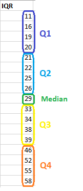
The interquartile range is the middle half of the data. To visualize it, think about the median value that splits the dataset in half. Similarly, you can divide the data into quarters. Statisticians refer to these quarters as quartiles and denote them from low to high as Q1, Q2, Q3, and Q4. The lowest quartile (Q1) contains the quarter of the dataset with the smallest values. The upper quartile (Q4) contains the quarter of the dataset with the highest values. The interquartile range is the middle half of the data that is in between the upper and lower quartiles. In other words, the interquartile range includes the 50% of data points that fall in Q2 and

The IQR is the red area in the graph below.

The interquartile range is a robust measure of variability in a similar manner that the median is a robust measure of central tendency. Neither measure is influenced dramatically by outliers because they don’t depend on every value. Additionally, the interquartile range is excellent for skewed distributions, just like the median. As you’ll learn, when you have a normal distribution, the standard deviation tells you the percentage of observations that fall specific distances from the mean. However, this doesn’t work for skewed distributions, and the IQR is a great alternative.

I’ve divided the dataset below into quartiles. The interquartile range (IQR) extends from the low end of Q2 to the upper limit of Q3. For this dataset, the range is 21 – 39.

Quartiles, Quartile Deviation and Quartile co-efficient

The Quartile Deviation is a simple way to estimate the spread of a distribution about a measure of its central tendency (usually the mean). So, it gives you an idea about the range within which the central 50% of your sample data lies. Consequently, based on the quartile deviation, the Coefficient of Quartile Deviation can be defined, which makes it easy to compare the spread of two or more different distributions. Since both of these topics are based on the concept of quartiles, we’ll first understand how to calculate the quartiles of a dataset before working with the direct formulae.

Quartiles

A median divides a given dataset (which is already sorted) into two equal halves similarly, the quartiles are used to divide a given dataset into four equal halves. Therefore, logically there should be three quartiles for a given distribution, but if you think about it, the second quartile is equal to the median itself! We’ll deal with the other two quartiles in this section.

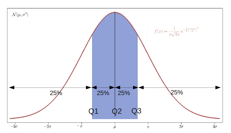
  • The first quartileor the lower quartile or the 25th percentile, also denoted by Q1corresponds to the value that lies halfway between the median and the lowest value in the distribution (when it is already sorted in the ascending order). Hence, it marks the region which encloses 25% of the initial data.
  • Similarly, the third quartileor the upper quartile or 75th percentile, also denoted by Q3, corresponds to the value that lies halfway between the median and the highest value in the distribution (when it is already sorted in the ascending order). It, therefore, marks the region which encloses the 75% of the initial data or 25% of the end data.

For a better understanding, look at the representation below for a Gaussian Distribution:

The Quartile Deviation

Formally, the Quartile Deviation is equal to the half of the Inter-Quartile Range and thus we can write it as:

Qd=(Q3–Q1)/2

Therefore, we also call it the Semi Inter-Quartile Range.

  • The Quartile Deviation doesn’t take into account the extreme points of the distribution. Thus, the dispersion or the spread of only the central 50% data is considered.
  • If the scale of the data is changed, the Qd also changes in the same ratio.
  • It is the best measure of dispersion for open-ended systems (which have open-ended extreme ranges).
  • Also, it is less affected by sampling fluctuations in the dataset as compared to the range (another measure of dispersion).
  • Since it is solely dependent on the central values in the distribution, if in any experiment, these values are abnormal or inaccurate, the result would be affected drastically.

The Coefficient of Quartile Deviation

Based on the quartiles, a relative measure of dispersion, known as the Coefficient of Quartile Deviation, can be defined for any distribution. It is formally defined as:

Coefficient of Quartile Deviation = {(Q3–Q1)/(Q3+Q1)}×100

Since it involves a ratio of two quantities of the same dimensions, it is unit-less. Thus, it can act as a suitable parameter for comparing two or more different datasets which may or may not involve quantities with the same dimensions.

So, now let’s go through the solved examples below to get a better idea of how to apply these concepts to various distributions.

Mean deviation with mean, Co-efficient of mean deviation

To understand the dispersion of data from a measure of central tendency, we can use mean deviation. It comes as an improvement over the range. It basically measures the deviations from a value. This value is generally mean or median. Hence although mean deviation about mode can be calculated, mean deviation about mean and median are frequently used.

Note that the deviation of an observation from a value a is d= x-aTo find out mean deviation we need to take the mean of these deviations. However, when this value of a is taken as mean, the deviations are both negative and positive since it is the central value.

This further means that when we sum up these deviations to find out their average, the sum essentially vanishes. Thus to resolve this problem we use absolute values or the magnitude of deviation. The basic formula for finding out mean deviation is :

Mean deviation= Sum of absolute values of deviations from ‘a’ ÷ The number of observations

Coefficient of Mean Deviation:

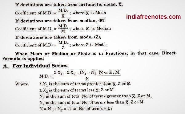
It is calculated to compare the data of two series. The coefficient of mean deviation is calculated by dividing mean deviation by the average. If deviations are taken from mean, we divide it by mean, if the deviations are taken from median, then it is divided by mode and if the “deviations are taken from median, then we divide mean deviation by median.

  1. For Discrete Series:

M.D. = ∑fdy/N; Where; N=∑f

And dy is the deviation of variable from X, M or Z ignoring signs (Taking +ive signs only).

Steps to Calculate:

  1. Take X, M or Z series as desired.
  2. Take deviations ignoring signs.
  3. Multiply dy by respective f; get ∑fdy
  4. Use the following formula

M.D. = ∑fdy/N

(Note : If value of X or M or Z is in decimal fractions better use Direct Method to get result easily)

When Mean or Median or Mode is in Fractions, in that case, Direct formula is applied

  1. For Continuous Series:

For Continuous Series also ;

M.D. = fdy/N

error: Content is protected !!