Tag: Regression Analysis

Conditional Probability refers to the probability of an event occurring given that another event has already occurred. It measures how the occurrence of one event affects the likelihood of another event. In many real-life situations, events are not independent, and the probability of one event depends on the outcome of another. Conditional probability helps analyze such relationships and provides a more accurate understanding of uncertain situations.

This concept is widely used in business, economics, finance, insurance, medicine, and statistics. It helps organizations make informed decisions by considering available information and understanding how different events are connected.

Definition

Conditional Probability is the probability of an event occurring under the condition that another related event has already taken place.

The probability of the occurrence of an event A given that an event B has already occurred is called the conditional probability of A given B:

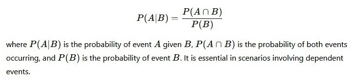
The same is explained in Figure 2.15 using the sample spaces related to the events A and B, assuming that there are few sample points common to these two events. Part 1 of the figure shows the total sample space related to the experiment as in the form of rectangle and the sample space related to the event A as a circle. Similarly part 2 of the figure shows the total sample space and the sample space related to event B. As explained earlier in conditional probability the total sample space is restrained to the sample space that is related to event B (which has already occurred). The same is shown in part 3 of Figure 2.15. Now the sample space for event A (B is the total sample space available) is nothing but the sample points related to event A and falling in the sample space. This is nothing but the intersection of the events A and B and is shown in part 3 of the figure as the hatched area.  

Figure 2.15: Representation of conditional probability using the Venn diagrams

For example, there are 100 trips per day between two places X and Y. Out of these 100 trips 50 are made by car, 25 are made by bus and the other 25 are by local train. Probabilities associated to these modes are 0.5, 0.25, and 0.25, respectively. In transportation engineering both the bus and the local train are considered as public transport so the event space associated to this is the summation of the event spaces associated to bus and local train. Probability of choosing public transportation is 0.5. Now if one is interested in finding the probability of choosing bus given public transportation is chosen the conditional probability is useful in finding that.

Characteristics of Conditional Probability

• Depends on the Occurrence of Another Event

A key characteristic of conditional probability is that it depends on the occurrence of another event. Unlike simple probability, which measures the likelihood of an event independently, conditional probability considers additional information. The probability of an event changes when another related event has already occurred. For example, the probability of a customer purchasing a printer may increase if the customer has already purchased a laptop. This dependency makes conditional probability highly useful in analyzing real-world situations where events are interconnected and influence one another.

• Measures Relationships Between Events

Conditional probability helps measure and understand the relationship between two or more events. It shows how the occurrence of one event affects the likelihood of another event occurring. By analyzing these relationships, businesses and researchers can identify patterns and dependencies within data. For example, a retailer may study whether customers who buy one product are more likely to buy another. This characteristic makes conditional probability valuable in market research, risk assessment, and forecasting. It provides insights into event interactions that simple probability cannot capture effectively.

• Based on Joint Probability

Another important characteristic is that conditional probability relies on joint probability. To calculate conditional probability, the probability of both events occurring together must be known. Joint probability provides the foundation for determining how likely one event is when another has already occurred. This relationship ensures that conditional probability is mathematically consistent and accurate. By using joint probability, analysts can examine event dependencies in a systematic manner. This characteristic highlights the close connection between different probability concepts and their role in statistical analysis.

• Applicable to Dependent Events

Conditional probability is particularly useful when dealing with dependent events. Dependent events are events where the occurrence of one influences the probability of another. In many business and real-world situations, events are not independent. For example, customer purchasing decisions may depend on previous purchases or promotional offers. Conditional probability helps quantify these dependencies and provides more realistic probability estimates. This characteristic makes it an essential tool for understanding situations where outcomes are interconnected and cannot be analyzed accurately using independent probabilities alone.

• Provides Updated Probability Estimates

Conditional probability allows probabilities to be updated when new information becomes available. Instead of relying solely on initial estimates, it incorporates additional data to produce revised probability values. This characteristic is especially important in dynamic environments where circumstances change over time. For example, a bank may reassess the probability of loan repayment after receiving updated information about a customer’s financial status. By adjusting probabilities based on current information, conditional probability improves the accuracy and relevance of decision-making and forecasting processes.

• Supports Better Decision-Making

A significant characteristic of conditional probability is its ability to support informed decision-making. By considering specific conditions and relevant information, it provides more accurate estimates of future outcomes. Managers, investors, and policymakers use conditional probability to evaluate alternatives and assess risks. For example, a business may determine the likelihood of achieving sales targets under certain market conditions. This information enables decision-makers to choose strategies that maximize opportunities and minimize risks. Consequently, conditional probability plays an important role in effective planning and management.

• Forms the Foundation of Advanced Statistical Methods

Conditional probability serves as the basis for many advanced statistical and analytical techniques. Concepts such as Bayes’ Theorem, predictive modeling, machine learning, and statistical inference all rely on conditional probability principles. By understanding how probabilities change under specific conditions, analysts can develop sophisticated models for forecasting and decision support. This characteristic demonstrates the importance of conditional probability in both theoretical and applied statistics. Its role as a foundational concept makes it essential for advanced research and data analysis across numerous disciplines.

• Widely Applicable in Real-Life Situations

Conditional probability has broad applicability in business, finance, insurance, healthcare, engineering, and many other fields. Real-world events are often dependent on specific conditions, making conditional probability highly relevant. Businesses use it to analyze customer behavior, assess risks, and forecast demand. Insurance companies use it to estimate claim probabilities based on customer profiles. Financial institutions apply it in credit risk analysis and investment decisions. This widespread applicability demonstrates its practical value and importance. As a result, conditional probability is one of the most widely used concepts in probability and statistics.

Applications of Conditional Probability in Business

Regression Line is the line that best fits the data, such that the overall distance from the line to the points (variable values) plotted on a graph is the smallest. In other words, a line used to minimize the squared deviations of predictions is called as the regression line.

There are as many numbers of regression lines as variables. Suppose we take two variables, say X and Y, then there will be two regression lines:

• Regression line of Y on X: This gives the most probable values of Y from the given values of X.
• Regression line of X on Y: This gives the most probable values of X from the given values of Y.

The algebraic expression of these regression lines is called as Regression Equations. There will be two regression equations for the two regression lines.

The correlation between the variables depend on the distance between these two regression lines, such as the nearer the regression lines to each other the higher is the degree of correlation, and the farther the regression lines to each other the lesser is the degree of correlation.

The correlation is said to be either perfect positive or perfect negative when the two regression lines coincide, i.e. only one line exists. In case, the variables are independent; then the correlation will be zero, and the lines of regression will be at right angles, i.e. parallel to the X axis and Y axis.

The regression lines cut each other at the point of average of X and Y. This means, from the point where the lines intersect each other the perpendicular is drawn on the X axis we will get the mean value of X. Similarly, if the horizontal line is drawn on the Y axis we will get the mean value of Y.

Co-efficient of Regression

The Regression Coefficient is the constant ‘b’ in the regression equation that tells about the change in the value of dependent variable corresponding to the unit change in the independent variable.

If there are two regression equations, then there will be two regression coefficients:

• Regression Coefficient of X on Y:

The regression coefficient of X on Y is represented by the symbol b_xy that measures the change in X for the unit change in Y. Symbolically, it can be represented as:

The b_xy can be obtained by using the following formula when the deviations are taken from the actual means of X and Y:When the deviations are obtained from the assumed mean, the following formula is used:

• Regression Coefficient of Y on X:

The symbol b_yx is used that measures the change in Y corresponding to the unit change in X. Symbolically, it can be represented as:

In case, the deviations are taken from the actual means; the following formula is used:
The _byx can be  calculated by using the following formula when the deviations are taken from the assumed means:

The Regression Coefficient is also called as a slope coefficient because it determines the slope of the line i.e. the change in the independent variable for the unit change in the independent variable

Scatter Diagram Method is the simplest method to study the correlation between two variables wherein the values for each pair of a variable is plotted on a graph in the form of dots thereby obtaining as many points as the number of observations. Then by looking at the scatter of several points, the degree of correlation is ascertained.

The degree to which the variables are related to each other depends on the manner in which the points are scattered over the chart. The more the points plotted are scattered over the chart, the lesser is the degree of correlation between the variables. The more the points plotted are closer to the line, the higher is the degree of correlation. The degree of correlation is denoted by “r”.

The following types of scatter diagrams tell about the degree of correlation between variable X and variable Y.

1. Perfect Positive Correlation (r = +1):

The correlation is said to be perfectly positive when all the points lie on the straight line rising from the lower left-hand corner to the upper right-hand corner.

2. Perfect Negative Correlation (r = -1):

When all the points lie on a straight line falling from the upper left-hand corner to the lower right-hand corner, the variables are said to be negatively correlated.

3. High Degree of +Ve Correlation (r = + High):

The degree of correlation is high when the points plotted fall under the narrow band and is said to be positive when these show the rising tendency from the lower left-hand corner to the upper right-hand corner.

4. High Degree of –Ve Correlation (r = – High):

The degree of negative correlation is high when the point plotted fall in the narrow band and show the declining tendency from the upper left-hand corner to the lower right-hand corner.

5. Low degree of +Ve Correlation (r = + Low):

The correlation between the variables is said to be low but positive when the points are highly scattered over the graph and show a rising tendency from the lower left-hand corner to the upper right-hand corner.

6. Low Degree of –Ve Correlation (r = + Low):

The degree of correlation is low and negative when the points are scattered over the graph and the show the falling tendency from the upper left-hand corner to the lower right-hand corner.

7. No Correlation (r = 0):

The variable is said to be unrelated when the points are haphazardly scattered over the graph and do not show any specific pattern. Here the correlation is absent and hence r = 0.

Thus, the scatter diagram method is the simplest device to study the degree of relationship between the variables by plotting the dots for each pair of variable values given. The chart on which the dots are plotted is also called as a Dotogram.

Mean Deviation

Mean deviation is a measure of dispersion that indicates the average of the absolute differences between each data point and the mean (or median) of the dataset. It provides an overall sense of how much the values deviate from the central value. To calculate mean deviation, the absolute differences between each data point and the central measure are summed and then divided by the number of observations. Unlike variance, mean deviation is expressed in the same units as the data and is less sensitive to extreme outliers.

The basic formula for finding out mean deviation is :

Mean Deviation = Sum of absolute values of deviations from ‘a’ ÷ The number of observations

Standard Deviation

Standard deviation is a widely used measure of dispersion that indicates the average amount by which each data point deviates from the mean. It is calculated by first finding the variance, which is the average of squared deviations, and then taking the square root of the variance. Standard deviation provides a more interpretable measure of spread, as it is in the same units as the original data. A higher standard deviation indicates greater variability, while a lower value indicates data points are closer to the mean, indicating less spread or consistency.

Usually represented by s or σ. It uses the arithmetic mean of the distribution as the reference point and normalizes the deviation of all the data values from this mean.

Therefore, we define the formula for the standard deviation of the distribution of a variable X with n data points as:

Median is a measure of central tendency that represents the middle value of an ordered dataset, dividing it into two equal halves. If the dataset has an odd number of values, the median is the middle value. If the dataset has an even number, it is the average of the two middle values. The median is less affected by outliers, making it useful for skewed data or non-uniform distributions.

Example:

The marks of nine students in a geography test that had a maximum possible mark of 50 are given below:

     47     35     37     32     38     39     36     34     35

Find the median of this set of data values.

Solution:

Arrange the data values in order from the lowest value to the highest value:

    32     34     35     35     36     37     38     39     47

The fifth data value, 36, is the middle value in this arrangement.

Characteristics of Median:

1. Middle Value of Data

The median divides a dataset into two equal halves, with 50% of the values lying below it and 50% above it. It is determined by arranging data in ascending or descending order.

2. Resistant to Outliers

The median is not influenced by extreme values or outliers. This makes it a more robust measure for datasets with significant variability or skewness.

3. Applicable to Ordinal and Quantitative Data

The median can be calculated for ordinal data (where data can be ranked) and quantitative data. It is not suitable for nominal data, as there is no inherent order.

4. Unique Value

For any given dataset, the median is always unique and provides a single central value, ensuring consistency in its interpretation.

5. Requires Data Sorting

The calculation of the median necessitates ordering the data values. Without arranging the data, the median cannot be identified.

6. Effective for Skewed Distributions

In skewed datasets, the median better represents the center compared to the mean, as it remains unaffected by the skewness.

7. Not Affected by Sample Size

Median’s calculation is straightforward and remains valid regardless of the sample size, as long as the data is properly ordered.

Applications of Median:

1. Income and Wealth Distribution

In economics and social studies, the median is used to analyze income and wealth distributions. For example, the median income indicates the income level at which half the population earns less and half earns more. It is more accurate than the mean in scenarios with extreme disparities, such as high-income earners skewing the average.

2. Real Estate Market Analysis

Median is commonly applied in the real estate industry to determine the central value of property prices. Median house prices are preferred over averages because they are less affected by outliers, such as extremely high or low-priced properties.

3. Educational Assessments

In education, the median is used to evaluate student performance. For example, the median test score helps identify the middle-performing student, providing a fair representation when the scores are unevenly distributed.

4. Medical and Health Statistics

Median is often employed in health sciences to summarize data such as median survival rates or recovery times. These metrics are crucial when the data includes extreme cases or a non-symmetric distribution.

5. Demographic Studies

Median age, household size, and other demographic measures are widely used in population studies. These metrics provide insights into the central characteristics of populations while avoiding distortion by extremes.

6. Transportation Planning

In transportation and traffic analysis, the median is used to determine the typical travel time or commute duration. It offers a realistic measure when the data includes unusually long or short travel times.

Demerits or Limitations of Median:

1. Even if the value of extreme items is too large, it does not affect too much, but due to this reason, sometimes median does not remain the representative of the series.
2. It is affected much more by fluctuations of sampling than A.M.
3. Median cannot be used for further algebraic treatment. Unlike mean we can neither find total of terms as in case of A.M. nor median of some groups when combined.
4. In a continuous series it has to be interpolated. We can find its true-value only if the frequencies are uniformly spread over the whole class interval in which median lies.

5. If the number of series is even, we can only make its estimate; as the A.M. of two middle terms is taken as Median.

Mode is a measure of central tendency that identifies the most frequently occurring value or values in a dataset. Unlike the mean or median, the mode can be used for both numerical and categorical data. A dataset may have one mode (unimodal), more than one mode (bimodal or multimodal), or no mode at all if no value repeats. The mode is particularly useful for understanding trends in categorical data, such as the most popular product, common response, or frequent event, and is less sensitive to outliers compared to other central tendency measures.

Examples:

For example, in the following list of numbers, 16 is the mode since it appears more times than any other number in the set:

• 3, 3, 6, 9, 16, 16, 16, 27, 27, 37, 48

A set of numbers can have more than one mode (this is known as bimodal if there are 2 modes) if there are multiple numbers that occur with equal frequency, and more times than the others in the set.

• 3, 3, 3, 9, 16, 16, 16, 27, 37, 48

In the above example, both the number 3 and the number 16 are modes as they each occur three times and no other number occurs more than that.

If no number in a set of numbers occurs more than once, that set has no mode:

• 3, 6, 9, 16, 27, 37, 48

Characteristics of Mode:

• Can Be Used for Qualitative and Quantitative Data

Mode can be applied to both qualitative (categorical) and quantitative data. For example, in market research, the mode can identify the most common product color or customer preference.

• Not Affected by Outliers

The mode is not influenced by extreme values or outliers in a dataset. For instance, in a dataset of salaries where most values are clustered around a certain range but a few extreme salaries exist, the mode will still reflect the most frequent salary, making it a useful measure when dealing with skewed data or anomalies.

• May Have Multiple Values

A dataset may have more than one mode. If there are two values that occur with the same highest frequency, the dataset is considered bimodal. If there are more than two, it is multimodal. In such cases, the mode provides insight into multiple frequent occurrences within the dataset, unlike the mean or median, which offer a single value.

• Can Be Uniquely Defined or Undefined

In some datasets, there may be no mode if all values occur with equal frequency. For example, in a dataset where every value appears only once, the mode is undefined. Conversely, in datasets with a clear most frequent value, the mode is uniquely defined.

• Easy to Calculate

The mode is simple to compute. It only requires identifying the value that appears most frequently in the dataset. No complex formulas or data manipulations are needed, making it a straightforward measure for quick analysis.

• Useful for Categorical Data

The mode is especially useful for categorical data where numerical calculations do not apply. For instance, in surveys where respondents choose their favorite color, the mode will show the most popular choice, providing valuable insights in marketing or social studies.

Applications of Mode:

1. Market Research

In market research, the mode is used to identify the most popular product, service, or customer preference. For example, if a survey is conducted to determine consumers’ favorite brands, the mode will highlight the brand chosen most frequently, helping businesses focus on popular trends.

2. Fashion and Retail Industry

The mode is widely used in the fashion and retail sectors to determine popular product styles, colors, or sizes. For example, if a clothing store wants to know the most commonly bought color of a particular item, the mode will provide the answer, guiding inventory decisions and promotional strategies.

3. Educational Testing

In educational assessments, the mode can be used to determine the most common score or grade achieved by students in a test or examination. This helps educators identify common performance trends and understand the difficulty level of the assessment.

4. Health and Medical Statistics

In healthcare, the mode is used to find the most common age group, symptom, or diagnosis within a population. For example, in a study of common diseases, the mode can reveal the most frequently occurring disease or the most prevalent age group affected, providing insights into public health needs.

5. Consumer Behavior Analysis

In consumer behavior studies, the mode is used to determine the most frequently chosen option in surveys and polls. For instance, it can highlight the most common reasons for customer dissatisfaction or preferences regarding product features, aiding companies in product development and customer service strategies.

6. Sports Statistics

In sports analytics, the mode is used to identify the most frequent performance metric. For example, the mode can be applied to identify the most common score in a set of matches or the most frequent outcome of a particular game, assisting coaches and analysts in understanding patterns in performance.

Advantages:

• It is easy to understand and simple to calculate.
• It is not affected by extremely large or small values.
• It can be located just by inspection in un-grouped data and discrete frequency distribution.
• It can be useful for qualitative data.
• It can be computed in an open-end frequency table.
• It can be located graphically.

Disadvantages:

• It is not well defined.
• It is not based on all the values.
• It is stable for large values so it will not be well defined if the data consists of a small number of values.
• It is not capable of further mathematical treatment.
• Sometimes the data has one or more than one mode, and sometimes the data has no mode at all.

Central Tendency is a statistical concept that identifies the central or typical value within a dataset, representing its overall distribution. It provides a single summary measure to describe the dataset’s center, enabling comparisons and analysis. The three primary measures of central tendency are:

1. Mean (Arithmetic Average): The sum of all values divided by the number of values.
2. Median: The middle value when data is ordered, dividing it into two equal halves.
3. Mode: The most frequently occurring value in the dataset.

Objectives of Measures of Central Tendency:

Measures of central tendency are statistical tools used to summarize and describe a dataset by identifying a central value that represents the data. These measures include the mean, median, and mode, each serving specific objectives to aid in data analysis.

1. Summarizing Data

The primary objective is to condense a large dataset into a single representative value. By calculating a central value, such as the mean, median, or mode, the complexity of raw data is reduced, making it easier to understand and interpret.

2. Identifying the Center of Distribution

Central tendency measures aim to determine the “center” or most typical value of a dataset. This central value acts as a benchmark around which data points are distributed, providing insights into the dataset’s overall structure.

3. Facilitating Comparisons

These measures allow comparisons between different datasets. For instance, comparing the mean income of two cities or the average performance of students across different schools can reveal relative trends and patterns.

4. Assisting in Decision-Making

Measures of central tendency provide essential information for making informed decisions. In business, knowing the average sales or customer preferences helps managers formulate strategies, allocate resources, and predict outcomes.

5. Assessing Data Symmetry and Distribution

The relationship between the mean, median, and mode can indicate the skewness of the data. For example:

• In symmetric distributions: Mean = Median = Mode.
• In positively skewed distributions: Mean > Median > Mode.
• In negatively skewed distributions: Mean < Median < Mode.

This helps in understanding the nature and spread of the dataset.

6. Comparing Groups within Data

Central tendency measures are crucial for comparing subsets within a dataset. For example, the average test scores of different age groups in a population can be compared to identify performance trends.

7. Highlighting Data Trends

These measures provide insights into recurring trends or patterns. For example, the mode identifies the most common value, which is useful in market research to understand consumer preferences.

8. Forming the Basis for Further Analysis

Central tendency measures serve as the foundation for advanced statistical analyses, such as variability, correlation, and regression. They provide an initial understanding of the dataset, guiding further exploration.