Author: indiafreenotes

A distributed database is basically a database that is not limited to one system, it is spread over different sites, i.e, on multiple computers or over a network of computers. A distributed database system is located on various sited that don’t share physical components. This maybe required when a particular database needs to be accessed by various users globally. It needs to be managed such that for the users it looks like one single database.

A distributed database is a collection of multiple interconnected databases, which are spread physically across various locations that communicate via a computer network.

Goals of Distributed Database system

The concept of distributed database was built with a goal to improve:

(i) Reliability

In distributed database system, if one system fails down or stops working for some time another system can complete the task.

(ii) Availability

In distributed database system reliability can be achieved even if sever fails down. Another system is available to serve the client request.

(iii) Performance

Performance can be achieved by distributing database over different locations. So the databases are available to every location which is easy to maintain.

Advantages of Distributed Databases

Following are the advantages of distributed databases over centralized databases.

(i) Modular Development

If the system needs to be expanded to new locations or new units, in centralized database systems, the action requires substantial efforts and disruption in the existing functioning. However, in distributed databases, the work simply requires adding new computers and local data to the new site and finally connecting them to the distributed system, with no interruption in current functions.

(ii) More Reliable

In case of database failures, the total system of centralized databases comes to a halt. However, in distributed systems, when a component fails, the functioning of the system continues may be at a reduced performance. Hence DDBMS is more reliable.

(iii) Better Response

If data is distributed in an efficient manner, then user requests can be met from local data itself, thus providing faster response. On the other hand, in centralized systems, all queries have to pass through the central computer for processing, which increases the response time.

(iv) Lower Communication Cost

In distributed database systems, if data is located locally where it is mostly used, then the communication costs for data manipulation can be minimized. This is not feasible in centralized systems.

Types of distributed database System

The two types of distributed systems are as follows:

1. Homogeneous distributed databases system

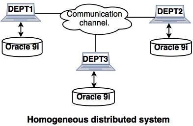
In a homogeneous database, all different sites store database identically. The operating system, database management system and the data structures used – all are same at all sites. Hence, they’re easy to manage.

Example: Consider that we have three departments using Oracle-9i for DBMS. If some changes are made in one department then, it would  update the other department also.

2. Heterogeneous Database

In a heterogeneous distributed database, different sites can use different schema and software that can lead to problems in query processing and transactions. Also, a particular site might be completely unaware of the other sites. Different computers may use a different operating system, different database application. They may even use different data models for the database. Hence, translations are required for different sites to communicate.

Example: In the following diagram, different DBMS software are accessible to each other  using ODBC and JDBC.

Distributed Data Storage

There are 2 ways in which data can be stored on different sites. These are:

1. Replication

In this approach, the entire relation is stored redundantly at 2 or more sites. If the entire database is available at all sites, it is a fully redundant database. Hence, in replication, systems maintain copies of data.

This is advantageous as it increases the availability of data at different sites. Also, now query requests can be processed in parallel.

However, it has certain disadvantages as well. Data needs to be constantly updated. Any change made at one site needs to be recorded at every site that relation is stored or else it may lead to inconsistency. This is a lot of overhead. Also, concurrency control becomes way more complex as concurrent access now needs to be checked over a number of sites.

2. Fragmentation

In this approach, the relations are fragmented (i.e., they’re divided into smaller parts) and each of the fragments is stored in different sites where they’re required. It must be made sure that the fragments are such that they can be used to reconstruct the original relation (i.e, there isn’t any loss of data).

Fragmentation is advantageous as it doesn’t create copies of data, consistency is not a problem.

Fragmentation of relations can be done in two ways:

• Horizontal fragmentation – Splitting by rows – The relation is fragmented into groups of tuples so that each tuple is assigned to at least one fragment.
• Vertical fragmentation – Splitting by columns – The schema of the relation is divided into smaller schemas. Each fragment must contain a common candidate key so as to ensure lossless join.

Security valuation is important to decide on the portfolio of an investor. All investment decisions are to be made on a scientific analysis of the right price of a share. Hence, an understanding of the valuation of securities is essential. Investors should buy underpriced shares and sell overpriced shares. Share pricing is thus an important aspect of trading. Conceptually, four types of valuation models are discernible.

They are:

(i) Book value,

(ii) Liquidating value,

(iii) Intrinsic value,

(iv) Replacement value as compared to market price.

(i) Book Value:

Book value of a security is an accounting concept. The book value of an equity share is equal to the net worth of the firm divided by the number of equity shares, where the net worth is equal to equity capital plus free reserves. The market value may fluctuate around the book value but may be higher if the future prospects are good.

(ii) Liquidating Value (Breakdown Value):

If the assets are valued at their breakdown value in the market and take net fixed assets plus current assets minus current liabilities as if the company is liquida­ted, then divide this by the number of shares, the resultant value is the liquidating value per share. This is also an accounting concept.

(iii) Intrinsic Value:

Market value of a security is the price at which the security is traded in the market and it is generally hovering around its intrinsic value. There are different schools of thought regarding the relationship of intrinsic value to the market price. Market prices are those which rule in the market, resulting from the demand and supply forces. Intrinsic price is the true value of the share, which depends on its earning capacity and its true worth. According to the fundamentalist approach to security valuation, the value of the security must be equal to the discounted value of the future income stream. The investor buys the securities when the market price is below this value.

Thus, for fundamentalists, earnings and dividends are the essential ingredients in determining the market value of a security. The discount rate used in such present value calculations is known as the required rate or return. Using this discount rate all future earnings are discounted back to the present to determine the intrinsic value.

According to the technical school, the price of a security is determined by the market demand and supply and it has very little to do with intrinsic values. The price movements follow certain trends for varying periods of time. Changes in trend represent the shifts in demand and supply which are predictable. The present trends are the offshoot of the past and history repeats itself according to this school.

According to efficient market hypothesis, in a fairly large security market where competitive conditions prevail, market prices are good proxies for intrinsic values. The security prices are determined after absorbing all the information avail­able to market participants. A share is thus generally worth whatever it is selling for in the market.

Generally, fundamental school is the basis for security valuation and many models are in use, based on these tenets.

(iv) Replacement Value:

When the company is liquidated and its assets are to be replaced by new ones, their prices being higher, the replacement value of a share will be different from the Breakdown value. Some analysts take this replacement value to compare with the market price.

Factors Influencing Security Valuation:

Security price depends on a host of factors like earnings per share, prospects of expansion, future earnings potential, possible issue of bonus or rights shares, etc. Some demand for a particular stock may give pleasure of power as a shareholder or prestige and control on management. Satisfaction and pleasure in the non-monetary sense cannot be considered in any practical and quantifiable sense. Many psychologi­cal and emotional factors influence the demand for a share.

In money terms, the return to a security on which its value depends consists of two components:

(i) Regular dividends or interest, and

(ii) Capital gains or losses in the form of changes in the capital value of the asset.

If the risk is high, return should also be high. Risk here refers to uncertainty of receipt of principal and interest or dividend and variability of this return.

The above returns are in terms of money received over a period of years. But money of Re. 1 received today is not the-same as money of Re. 1 received a year hence or two years hence etc. Money has time value, which suggests that earlier receipts are more desirable and valuable than later receipts. One reason for this is that earlier receipts can be reinvested and more receipts can be got than before. Here the principle operating is compound interest.

Thus, if Vn is the terminal value at the period n, P is the initial value, g is rate of compounding or return, n is the number of compounding periods, then Vn = P (1 + g)ⁿ.

If we reverse the process, the present value (P) can be thought of as reversing the compounding of values. This is discounting of the future values to the present day, represented by the formula-

P = Vn /(1+ g)ⁿ

Graham’s Approach to Valuation of Equity:

In their book on Security Analysis (1934) Benjamin Graham, and David Dodd, argued that future earnings power was the most important determinant of the value of stock. The original approach of identifying the undervalued stock is to find out the present value of forecasted dividends, and if the current market price is lower, it is undervalued. Alternatively, the analyst could determine the discount rate that makes the present value of the forecasted dividends equal to the current market price of the stock. If that rate (I.R.R. or discount rate) is more than the required rate for stocks of similar risks, then the stock is underpriced.

Graham and Dodd had argued that each dollar of dividends is worth four times as much as one dollar of retained earnings (in their original Book); but subsequent studies of data showed no justification for this. Graham and Rea have given some questions on Rewards and risks for financial data analysts to answer yes or no and on the basis of these ready to answer questions, they decided to locate undervalued stocks to buy and overvalued stocks to sell.

Such readymade formulas or questions are now out of favour due to various empirical studies which showed that earnings models are as good as or better than dividend models and that a number of factors are ably studied for common stock valuation and no unique formula or answer is justifiable.

Securities Valuation in India:

In India, the valuation of securities used to be done by the CCI for the purpose of fixing up the premium on new issues of existing companies. These guidelines used by CCI were applicable upto May 1992, when the CCI was abolished. Although the present market price will be taken into account a more rational price used to be worked out by the CCI on certain criteria.

Thus, the CCI used the concept of Net Asset Value (NAV) and Profit-Earning Capacity Value (PECV) as the basis for fixing up the premium on shares. The NAV is calculated by dividing the net worth by the number of equity shares. The net worth includes equity capital plus free reserves and surplus less contingent liabilities.

The method for valuation of bonds involves three steps as follows:

Step 1: Estimate the expected cash flows

Step 2: Determine the appropriate interest rate that should be used to discount the cash flows.

& Step 3: Calculate the present value of the expected cash flows (step-1) using appropriate interest rate (step- 2) i.e. discounting the expected cash flows

STEP 1: Estimating cash flows

Cash flow is the cash that is estimated to be received in future from investment in a bond. There are only two types of cash flows that can be received from investment in bonds i.e. coupon payments and principal payment at maturity.

The usual cash flow cycle of the bond is coupon payments are received at regular intervals as per the bond agreement, and final coupon plus principle payment is received at the maturity. There are some instances when bonds don’t follow these regular patterns. Unusual patterns maybe a result of the different type of bond such as zero-coupon bonds, in which there are no coupon payments. Considering such factors, it is important for an analyst to estimate accurate cash flow for the purpose of bond valuation.

STEP 2: Determine the appropriate interest rate to discount the cash flows

Once the cash flow for the bond is estimated, the next step is to determine the appropriate interest rate to discount cash flows. The minimum interest rate that an investor should require is the interest available in the marketplace for default-free cash flow. Default-free cash flows are cash flows from debt security which are completely safe and has zero chances default. Such securities are usually issued by the central bank of a country, for example, in the USA it is bonds by U.S. Treasury Security.

Consider a situation where an investor wants to invest in bonds. If he is considering to invest corporate bonds, he is expecting to earn higher return from these corporate bond compared to rate of returns of U.S. Treasury Security bonds. This is because chances are that a corporate bond might default, whereas the U.S. Security Treasury bond is never going to default. As he is taking a higher risk by investing in corporate bonds, he expects a higher return.

One may use single interest rate or multiple interest rates for valuation.

STEP 3: Discounting the expected cash flows

Now that we already have values of expected future cash flows and interest rate used to discount the cash flow, it is time to find the present value of cash flows. Present Value of a cash flow is the amount of money that must be invested today to generate a specific future value. The present value of a cash flow is more commonly known as discounted value.

The present value of a cash flow depends on two determinants:

• When a cash flow will be received i.e. timing of a cash flow
• The required interest rate, more widely known as Discount Rate (rate as per Step-2)

First, we calculate the present value of each expected cash flow. Then we add all the individual present values and the resultant sum is the value of the bond.

The formula to find the present value of one cash flow is:

PRESENT VALUE FORMULA FOR BOND VALUATION

Present Value _n = Expected cash flow in the period n/ (1+i) ⁿ

Here,

i = rate of return/discount rate on bond
n = expected time to receive the cash flow

By this formula, we will get the present value of each individual cash flow t years from now. The next step is to add all individual cash flows.

Bond Value = Present Value ₁ + Present Value ₂ + ……. + Present Value _n

One of the most important skills an investor can learn is how to value a stock. It can be a big challenge though, especially when it comes to stocks that have supernormal growth rates. These are stocks that go through rapid growth for an extended period of time, say, for a year or more.

Many formulas in investing, though, are a little too simplistic given the constantly changing markets and evolving companies. Sometimes when you’re presented with a growth company, you can’t use a constant growth rate. In these cases, you need to know how to calculate value through both the company’s early, high growth years, and its later, lower constant growth years. It can mean the difference between getting the right value or losing your shirt.

Supernormal Growth Model

The supernormal growth model is most commonly seen in finance classes or more advanced investing certificate exams. It is based on discounting cash flows. The purpose of the supernormal growth model is to value a stock that is expected to have higher than normal growth in dividend payments for some period in the future. After this supernormal growth, the dividend is expected to go back to normal with constant growth.

To understand the supernormal growth model we will go through three steps:

• Dividend discount model (no growth in dividend payments)
• Dividend growth model with constant growth (Gordon Growth Model)
• Dividend discount model with supernormal growth

Dividend Discount Model: No Dividend Payments Growth

Preferred equity will usually pay the stockholder a fixed dividend, unlike common shares. If you take this payment and find the present value of the perpetuity, you will find the implied value of the stock.

For example, if ABC Company is set to pay a $1.45 dividend during the next period and the required rate of return is 9%, then the expected value of the stock using this method would be $1.45/0.09 = $16.11. Every dividend payment in the future was discounted back to the present and added together.

We can use the following formula to determine this model:

V= Dn/K

Where:

V=Value

Dn​=Dividend in the next period

k= Required rate of return​

Constant Growth Model: Gordon Growth Model

Next, let’s assume there is a constant growth in the dividend. This would be best suited for evaluating larger, stable dividend-paying stocks. Look to the history of consistent dividend payments and predict the growth rate given the economy the industry and the company’s policy on retained earnings.

Again, we base the value on the present value of future cash flows:

V = D1/ (k-g)

Where:

V=Value

D1=Dividend in the first period

k= Required rate of return

g=Dividend growth rate​

Dividend Discount Model with Supernormal Growth

Now that we know how to calculate the value of a stock with a constantly growing dividend, we can move on to a supernormal growth dividend.

One way to think about the dividend payments is in two parts: A and B. Part A has a higher growth dividend, while Part B has a constant growth dividend.

A) Higher Growth

This part is pretty straight forward. Calculate each dividend amount at the higher growth rate and discount it back to the present period. This takes care of the supernormal growth period. All that is left is the value of the dividend payments which will grow at a continuous rate.

B) Regular Growth

Still working with the last period of higher growth, calculate the value of the remaining dividends using the V = D₁ ÷ (k – g) equation from the previous section. But D₁, in this case, would be next year’s dividend, expected to be growing at the constant rate. Now the discount goes back to the present value through four periods.

A common mistake is discounting back five periods instead of four. But we use the fourth period because the valuation of the perpetuity of dividends is based on the end of year dividend in period four, which takes into account dividends in year five and on.

The values of all discounted dividend payments are added up to get the net present value. For example, if you have a stock that pays a $1.45 dividend which is expected to grow at 15% for four years, then at a constant 6% into the future, the discount rate is 11%.

An annuity due is a series of equal consecutive payments that you are either paying as a debtor or receiving as a lender. This differs from an annuity, as an annuity is a form of investment. Annuities are paid at the end of a period, while an annuity due payment is made at the beginning of a period. This payment covers the period to come.

Some examples of this could be a premium on insurance or rent due. If you were renting a house to someone, their monthly payments are an annuity due.

Time Value of Money 

Present value can be a difficult topic to digest. It refers to a concept called “the time value of money”. Time value of money can be explained thusly—if you were given $1 today, it is worth more than the same $1 five years from now. This is due to the changing value of money and inflation, and the potential of money to earn interest.

The present value of an annuity due (PVAD) is calculating the value at the end of the number of periods given, using the current value of money. Another way to think of it is how much an annuity due would be worth when payments are complete in the future, brought to the present.

Calculating the PVAD

For this formula, the following values are used:

P = periodic payment

r = rate per period

n = number of periods

The formula used is:

PVAD = P + P [ (1 – (1 + r) ^{– (n – 1)} ) ÷ r ]

An annuity is essentially a finance related contract, which permits the person who is buying it to pay on a lump-sum basis or make payments in series, in return for acquiring disbursements at regular intervals in future. Deferred Payment Annuity is a type of an annuity in which the payments that are received start somewhere in the future instead of starting at the time it is initiated.

Deferred payment annuity generally provides tax-deferred development and growth at a variable or fixed rate of return, similar to a regular annuity. Deferred payment annuity is usually bought for under-age or small children so that the benefit payment amount can be postponed till they complete a certain or desired age. Such annuities are extremely helpful when it comes to planning for retirement.

Deferred annuities are a type of annuity contract that delays payments to the investor until the investor elects to receive them. When the investor is in savings mode, he makes payments into some sort of investment account. The investment grows and compounds in a tax-deferred manner, and the investor pays no taxes on its growth until he decides to convert the investment into an annuity and start receiving regular payments.

A deferred annuity is essentially an investment vehicle that is sold by companies that provide insurance to people. The value of a deferred annuity can typically be calculated in two different ways i.e. future based value or present based value. It is these particular values that can assist you in determining the amount you should invest in order to fulfill your investment related goals.

Deferred annuity formula is used to calculate the present value of the deferred annuity which is promised to be received after some time and it is calculated by determining the present value of the payment in the future by considering the rate of interest and period of time.

Present Value Calculation

As per this method, you need to take the present value i.e. the amount you are thinking of investing today, into consideration. Next, you will have to provide definitions for the variables. For example, if you wish to make a saving of 100,000 dollars by the time a decade comes to an end and you come across an annuity that would offer you a minimum of 5% return on an annual basis, then your present value would typically be a minimum of 61,391 dollars today.

Future Value Calculation

For this, you will have to make note of the future value, which is the amount that you would receive after the maturity of the annuity. Next, define all the variables. For example, if you are planning to make an investment of 10,000 dollars and wish to find out how your asset would grow in case you were to get a 5% rate of interest over a period of twenty years, then your investment’s future value would be 26,532 dollars.

An annuity is the series of periodic payments received by an investor on a future date and the term “deferred annuity” refers to the delayed annuity in the form of installment or lump-sum payments rather than an immediate stream of income. It is basically the present value of the future annuity payment. The formula for a deferred annuity based on an ordinary annuity (where the annuity payment is done at the end of each period) is calculated using ordinary annuity payment, the effective rate of interest, number of periods of payment and deferred periods.

Deferred Annuity = P _Ordinary * [1 – (1 + r)^-n] / [(1 + r)^t * r]

A perpetuity is a type of annuity that receives an infinite amount of periodic payments. An annuity is a financial instrument that pays consistent periodic payments. As with any annuity, the perpetuity value formula sums the present value of future cash flows.

Common examples of when the perpetuity value formula is used is in consols issued in the UK and preferred stocks. Preferred stocks in most circumstances receive their dividends prior to any dividends paid to common stocks and the dividends tend to be fixed, and in turn, their value can be calculated using the perpetuity formula.

The value of a perpetuity can change over time even though the payment remains the same. This occurs as the discount rate used may change. If the discount rate used lowers, the denominator of the formula lowers, and the value will increase.

It should be noted that the formula shown supposes that the cash flows per period never change.