Month: April 2020

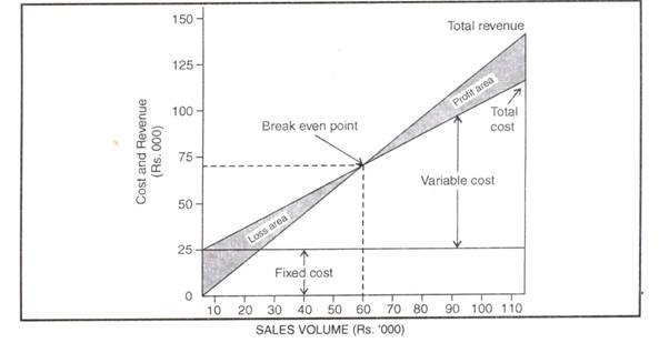
Break-Even Analysis is a financial and risk analysis technique used to determine the level of sales, production, or revenue at which a project or business neither earns a profit nor incurs a loss. The point at which total revenue equals total cost is known as the Break-Even Point (BEP). In capital budgeting, break-even analysis helps managers assess the minimum level of performance required for a project to recover its costs and become financially viable.

This technique is useful for evaluating project risk because it shows how sensitive profitability is to changes in sales volume, costs, or prices. A project with a lower break-even point is generally considered less risky because it can cover its costs with lower sales. Therefore, break-even analysis is an important tool for investment planning, pricing decisions, cost control, and risk assessment.

Formula of Break-Even Analysis

Break-Even Point (Units)

BEP (Units) = Fixed Costs ÷ Contribution per Unit

Where:

Contribution per Unit = Selling Price per Unit − Variable Cost per Unit

Break – Even Point (Sales Value)

BEP (Sales) = Fixed Costs ÷ P/V Ratio

Where:

P/V Ratio = Contribution ÷ Sales × 100

Example of Break-Even Analysis

Suppose:

• Fixed Costs = ₹2,00,000
• Selling Price per Unit = ₹100
• Variable Cost per Unit = ₹60

Step 1: Calculate Contribution per Unit

Contribution = ₹100 − ₹60

Contribution = ₹40

Step 2: Calculate Break-Even Point

BEP = ₹2,00,000 ÷ ₹40

BEP = 5,000 Units

Interpretation: The company must sell 5,000 units to cover all costs. Sales beyond this point will generate profit.

Features of Break-Even Analysis

• Identifies the No-Profit No-Loss Point

A major feature of break-even analysis is that it identifies the no-profit no-loss point of a business or project. This point is known as the break-even point, where total revenue equals total costs. At this stage, the organization neither earns a profit nor incurs a loss. It helps managers understand the minimum level of sales or production required to recover all fixed and variable costs. By determining this critical point, businesses can establish realistic sales targets and evaluate whether a project is financially feasible before committing resources to long-term investments.

• Measures the Risk Level of a Project

Break-even analysis serves as an effective tool for measuring project risk. A project with a high break-even point requires greater sales to cover costs and is therefore considered riskier. Conversely, a lower break-even point indicates lower risk because fewer sales are needed to avoid losses. This feature helps managers assess the financial vulnerability of investment projects. By understanding how much sales volume is necessary to reach profitability, organizations can evaluate whether projected demand is sufficient and make informed decisions regarding project acceptance or rejection.

• Focuses on Cost-Volume-Profit Relationship

An important feature of break-even analysis is its emphasis on the relationship between costs, sales volume, and profits. It examines how changes in production levels, selling prices, fixed costs, and variable costs affect profitability. This cost-volume-profit relationship helps managers understand the impact of operational decisions on financial performance. By analyzing these relationships, businesses can identify the most profitable production and sales levels. This feature makes break-even analysis a valuable planning and control tool for improving efficiency, maximizing profits, and managing business operations effectively.

• Helps in Profit Planning

Break-even analysis is useful not only for identifying the no-profit no-loss point but also for profit planning. Once the break-even point is known, managers can determine the level of sales required to achieve specific profit targets. This feature helps organizations set realistic revenue goals and evaluate whether projected sales volumes are sufficient to generate desired returns. Profit planning through break-even analysis supports strategic decision-making and helps businesses align operational activities with financial objectives. As a result, it contributes to improved profitability and long-term business success.

• Assists in Pricing Decisions

Another significant feature of break-even analysis is its role in pricing decisions. By understanding the relationship between selling price, costs, and profitability, managers can determine appropriate pricing strategies. If costs increase, break-even analysis helps estimate how much the selling price should be adjusted to maintain profitability. Similarly, it assists in evaluating the impact of price reductions on sales requirements and profits. This feature enables businesses to make informed pricing decisions that balance competitiveness with financial sustainability, ensuring that products remain profitable while meeting market demands.

• Facilitates Cost Control

Break-even analysis provides valuable insights into cost behavior and facilitates effective cost control. It separates costs into fixed and variable components, helping managers understand how each type of cost affects profitability. By analyzing cost structures, businesses can identify opportunities to reduce unnecessary expenses and improve operational efficiency. This feature supports better resource utilization and helps maintain financial stability. Effective cost control through break-even analysis contributes to lower break-even points, increased profitability, and improved competitiveness in the market, making it an essential tool for financial management.

• Simple and Easy to Understand

One of the key features of break-even analysis is its simplicity. The method is easy to understand and apply because it uses basic financial information such as costs, sales prices, and production volumes. Managers, investors, and students can easily interpret the results without requiring advanced statistical knowledge. Graphical representations such as break-even charts further enhance understanding by visually showing the relationship between costs, revenue, and profits. This simplicity makes break-even analysis a widely used tool for evaluating business performance, planning operations, and making investment decisions.

• Useful for Planning and Decision Making

Break-even analysis is an important planning and decision-making tool. It provides valuable information about the sales volume required to cover costs and achieve profitability. Managers use this information when evaluating investment projects, expanding operations, introducing new products, or making production decisions. The analysis helps compare different alternatives and assess their financial implications. By providing a clear understanding of cost and revenue relationships, break-even analysis supports informed decision-making and reduces uncertainty. This feature makes it an essential component of financial planning, budgeting, and strategic business management.

Methods of Break Even Analysis

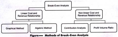
1. Graphical Method of Break-Even Analysis

The Graphical Method is a visual technique used to determine the break-even point through a chart known as the Break-Even Chart. In this method, sales volume is represented on the horizontal (X) axis, while costs and revenue are represented on the vertical (Y) axis. Separate lines are drawn for total cost and total revenue. The point where these two lines intersect is called the Break-Even Point (BEP). At this point, total revenue equals total cost, resulting in neither profit nor loss.

The graphical method provides a clear visual representation of profits, losses, and the margin of safety. It helps managers easily understand the relationship between costs, sales, and profitability. Although simple and effective, it may become less accurate when dealing with multiple products or complex cost structures.

Steps in the Graphical Method

• Draw X-axis for sales volume and Y-axis for costs and revenue.
• Plot the fixed cost line.
• Plot the total cost line (Fixed Cost + Variable Cost).
• Plot the total revenue line.
• Identify the intersection point of total cost and total revenue.
• The intersection point represents the Break-Even Point.

Formula Used

Break-Even Point (Units) = Fixed Costs ÷ Contribution per Unit

Example

• Fixed Costs = ₹1,50,000
• Selling Price per Unit = ₹100
• Variable Cost per Unit = ₹70

Contribution per Unit

= ₹100 − ₹70

= ₹30

Break-Even Point

= ₹1,50,000 ÷ ₹30

= 5,000 Units

On the graph, the Total Revenue Line and Total Cost Line intersect at 5,000 units, indicating the break-even point.

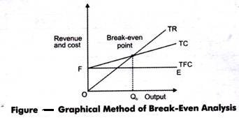
As shown in Fig. TFC is equals to FE, which is a fixed cost line. The vertical distance between TC and TFC line equals TVC. As quantity of output increases, the vertical distance between TC and TFC increases. This implies that TVC increases with change in TC and TFC.

Until Qb of the quantity is produced, total cost exceeds the total revenue, which implies that an organization will suffer losses if it produces less than Qb. At Qb output level, total revenue equals total cost. At this point, an organization never makes profit nor loss implying that it is a break-even point. Thus, Qb is a break-even level of output. Producing more than Qb will be profitable for organizations as TR is greater than TC.

2. Algebraic Method of Break-Even Analysis

The Algebraic Method is a mathematical approach used to calculate the break-even point using formulas. It determines the level of sales or production where total revenue equals total cost. This method is more accurate than the graphical method because it provides exact numerical results. It is widely used in financial planning, budgeting, and capital budgeting decisions.

The algebraic method is based on the concept of contribution margin, which is the difference between selling price and variable cost per unit. By dividing fixed costs by contribution per unit, managers can determine the number of units that must be sold to cover all costs. This method is simple, reliable, and suitable for business decision-making.

Formula: Break-Even Point (Units)

BEP = Fixed Costs ÷ Contribution per Unit

Where:

Contribution per Unit = Selling Price − Variable Cost

Break-Even Point (Sales Value)

BEP (Sales) = Fixed Costs ÷ P/V Ratio

Where:

P/V Ratio = (Contribution ÷ Sales) × 100

Example

• Fixed Costs = ₹2,00,000
• Selling Price per Unit = ₹120
• Variable Cost per Unit = ₹80

Step 1: Calculate Contribution

Contribution per Unit

= ₹120 − ₹80

= ₹40

Step 2: Calculate Break-Even Point

BEP

= ₹2,00,000 ÷ ₹40

= 5,000 Units

Interpretation: The company must sell 5,000 units to cover all fixed and variable costs. Any sales beyond this level will generate profit.

3. Contribution Margin Method

The Contribution Margin Method determines the break-even point by calculating the contribution made by each unit sold toward covering fixed costs. Contribution is the difference between selling price and variable cost per unit. Once fixed costs are fully covered, the remaining contribution becomes profit. This method is widely used because it directly focuses on the profitability of individual products and helps managers evaluate pricing and production decisions.

Formula

Contribution per Unit = Selling Price − Variable Cost

Break-Even Point (Units) = Fixed Costs ÷ Contribution per Unit

Example

• Fixed Costs = ₹2,00,000
• Selling Price = ₹100
• Variable Cost = ₹60

Contribution = ₹40

Break-Even Point

= ₹2,00,000 ÷ ₹40

= 5,000 Units

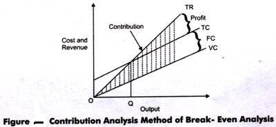
Fixed costs are addition to variable costs. Thus, TC line is parallel to the variable costs line. In the fig. OQ is the break-even point. TC minus VC equals FC. Below OQ, contribution is less than fixed cost whereas beyond OQ, contribution exceeds faxed cost. The shaded portion between TR and VC is the contribution.

4. Profit-Volume (P/V) Ratio Method

The Profit-Volume Ratio Method uses the contribution-to-sales relationship to determine the break-even point. The P/V ratio indicates how much contribution is generated from each rupee of sales. A higher P/V ratio indicates better profitability and a lower break-even point. This method is particularly useful for comparing products and evaluating the effect of changes in price and costs on profitability.

Formula

P/V Ratio = (Contribution ÷ Sales) × 100

Break-Even Sales = Fixed Costs ÷ P/V Ratio

Example

• Sales = ₹5,00,000
• Contribution = ₹2,00,000
• Fixed Costs = ₹80,000

P/V Ratio

= (2,00,000 ÷ 5,00,000) × 100

= 40%

Break-Even Sales

= ₹80,000 ÷ 40%

= ₹2,00,000

5. Margin of Safety Method

The Margin of Safety Method measures the difference between actual sales and break-even sales. It indicates the extent to which sales can decline before the business starts incurring losses. A higher margin of safety suggests lower risk, while a lower margin indicates greater financial vulnerability. This method helps managers evaluate business stability and assess the risk associated with sales fluctuations.

Formula: Margin of Safety = Actual Sales − Break-Even Sales

Margin of Safety Ratio = (Margin of Safety ÷ Actual Sales) × 100

Example

• Actual Sales = ₹8,00,000
• Break-Even Sales = ₹5,00,000

Margin of Safety

= ₹8,00,000 − ₹5,00,000

= ₹3,00,000

Margin of Safety Ratio

= (₹3,00,000 ÷ ₹8,00,000) × 100

= 37.5%

6. Cash Break-Even Analysis

Cash Break-Even Analysis focuses only on cash expenses and excludes non-cash costs such as depreciation. It determines the level of sales required to cover cash operating costs. This method is particularly useful for evaluating liquidity and ensuring that the business can meet its cash obligations. It is often used in project appraisal and financial planning where cash flow considerations are important.

Formula: Cash Break-Even Point = Cash Fixed Costs ÷ Contribution per Unit

Example

• Cash Fixed Costs = ₹1,20,000
• Contribution per Unit = ₹40

Cash Break-Even Point

= ₹1,20,000 ÷ ₹40

= 3,000 Units

This means the business must sell 3,000 units to cover all cash expenses.

7. Multi-Product Break-Even Analysis

Multi-Product Break-Even Analysis is used when a company sells more than one product. Since different products have different contribution margins, a weighted average contribution is calculated. This method helps determine the combined sales level required to achieve break-even for the entire product mix. It is particularly useful for diversified businesses with multiple product lines.

Formula: Break-Even Point = Fixed Costs ÷ Weighted Average Contribution

Example

• Fixed Costs = ₹4,00,000
• Weighted Average Contribution = ₹80

Break-Even Point

= ₹4,00,000 ÷ ₹80

= 5,000 Units

The company must collectively sell 5,000 units of its product mix to break even.

8. Analytical Break-Even Method

The Analytical Break-Even Method combines financial calculations and managerial analysis to determine the break-even point and evaluate profitability. It considers changes in costs, prices, production levels, and market conditions. This method provides a deeper understanding of financial performance and supports strategic decision-making. Managers often use it for long-term planning and evaluating alternative business strategies.

Formula: Break-Even Point = Fixed Costs ÷ Contribution Margin

Example

• Fixed Costs = ₹3,00,000
• Contribution Margin = ₹60 per unit

Break-Even Point

= ₹3,00,000 ÷ ₹60

= 5,000 Units

This analysis helps managers understand how operational changes affect profitability and risk.

Importance of Break-Even Analysis

• Helps in Determining Minimum Sales Requirement

Break-even analysis helps businesses determine the minimum level of sales required to cover all fixed and variable costs. By identifying the break-even point, managers can set realistic sales targets and ensure that operations remain financially sustainable. It provides a clear understanding of how much revenue is needed before profits can be earned. This information is particularly useful for new businesses and investment projects, as it helps assess feasibility and financial viability. Therefore, break-even analysis serves as an essential tool for planning sales strategies and avoiding potential losses.

• Assists in Profit Planning

A significant importance of break-even analysis is its role in profit planning. Once the break-even point is known, managers can estimate the additional sales required to achieve specific profit objectives. This enables businesses to establish realistic financial goals and develop strategies to attain them. Profit planning also helps in budgeting, forecasting, and evaluating future business performance. By understanding the relationship between sales volume and profitability, organizations can make better operational decisions. Thus, break-even analysis supports effective profit management and contributes to long-term financial success.

• Facilitates Pricing Decisions

Break-even analysis plays an important role in determining appropriate pricing policies. It helps managers understand how changes in selling prices affect profitability and the break-even point. If production costs increase, businesses can evaluate whether price adjustments are necessary to maintain profits. Similarly, before offering discounts or promotional pricing, managers can assess the impact on sales requirements. This information helps organizations balance competitiveness and profitability. Therefore, break-even analysis provides valuable guidance for setting prices that support both market demand and financial objectives.

• Supports Cost Control

Another important benefit of break-even analysis is its contribution to cost control. By separating costs into fixed and variable components, it helps managers identify areas where expenses can be reduced. Understanding cost behavior allows businesses to improve operational efficiency and manage resources more effectively. Cost control is essential for lowering the break-even point and increasing profitability. Managers can evaluate the impact of cost-saving measures and make informed decisions regarding production processes. Consequently, break-even analysis promotes better financial management and enhances the overall performance of the organization.

• Measures Business Risk

Break-even analysis is an effective tool for measuring the risk associated with a business or project. A high break-even point indicates greater risk because higher sales volumes are required to cover costs. Conversely, a lower break-even point suggests lower risk and greater financial stability. By assessing risk levels, managers can evaluate the feasibility of investment projects and make informed decisions. This understanding helps businesses prepare for market fluctuations and economic uncertainties. Therefore, break-even analysis contributes significantly to risk assessment and financial planning.

• Aids in Capital Budgeting Decisions

In capital budgeting, break-even analysis helps managers evaluate investment projects by estimating the sales volume needed to recover costs. It provides valuable information about project feasibility and profitability before large investments are made. By comparing the break-even points of different projects, businesses can select the most suitable investment opportunities. This analysis reduces uncertainty and improves decision-making regarding long-term investments. As a result, break-even analysis supports efficient allocation of resources and contributes to the achievement of organizational objectives.

• Assists in Business Planning and Forecasting

Break-even analysis is an important planning and forecasting tool. It helps businesses estimate future sales requirements, revenue targets, and production levels. Managers can use the information to prepare budgets, allocate resources, and develop strategic plans. Forecasting future performance becomes easier when the relationship between costs, sales, and profits is clearly understood. This enables organizations to anticipate challenges and respond proactively to changing market conditions. Therefore, break-even analysis enhances planning accuracy and supports effective business management.

• Improves Decision Making

One of the greatest advantages of break-even analysis is that it improves managerial decision-making. It provides reliable information regarding costs, revenues, profitability, and risk, enabling managers to make informed choices. Decisions related to pricing, production, expansion, product launches, and investment projects can be evaluated more effectively using break-even analysis. By reducing uncertainty and providing a clear financial picture, it enhances confidence in decision-making. Consequently, break-even analysis contributes to better financial performance, efficient resource utilization, and sustainable business growth.

Limitations of Break-Even Analysis

• Assumes Constant Selling Price

One major limitation of break-even analysis is that it assumes the selling price of a product remains constant at all levels of sales. In reality, businesses often change prices due to competition, market demand, discounts, seasonal variations, and economic conditions. A reduction in selling price can increase the break-even point, while a price increase may reduce it. Since actual market conditions rarely remain stable, this assumption limits the accuracy of break-even analysis. Therefore, the results obtained may not always reflect real business situations and profitability levels.

• Assumes Fixed and Variable Costs Remain Constant

Break-even analysis assumes that fixed costs and variable costs remain unchanged over the relevant range of production and sales. However, in practice, costs may change due to inflation, wage increases, changes in raw material prices, technological developments, or operational inefficiencies. Fixed costs may rise with business expansion, and variable costs may fluctuate depending on production volume. Because cost behavior is not always stable, the assumptions of break-even analysis may not accurately represent actual business conditions. This reduces its reliability for long-term financial planning and decision-making.

• Ignores Changes in Market Conditions

Another limitation of break-even analysis is that it does not consider changing market conditions. Factors such as competition, consumer preferences, economic cycles, government policies, and technological developments can significantly affect sales and profitability. The analysis assumes that products can be sold at expected levels without considering market uncertainties. In reality, businesses operate in dynamic environments where demand and supply conditions continuously change. Since break-even analysis ignores these external influences, it provides only a simplified view of profitability and may lead to inaccurate conclusions.

• Assumes All Units Produced Are Sold

Break-even analysis assumes that all units produced are sold immediately. This assumption simplifies calculations but does not always reflect actual business operations. Companies often maintain inventories due to seasonal demand, production scheduling, or market conditions. Unsold goods increase storage costs and affect cash flows. If production exceeds sales, the break-even calculations may not accurately indicate profitability. Therefore, the assumption that production and sales volumes are equal limits the practical applicability of break-even analysis, especially in businesses where inventory management plays a significant role.

• Not Suitable for Multi-Product Businesses

Break-even analysis is relatively simple when a company produces a single product. However, it becomes more complicated when multiple products with different selling prices, costs, and contribution margins are involved. In such cases, determining a single break-even point requires assumptions regarding product mix and sales proportions. Changes in the sales mix can significantly affect profitability and break-even calculations. Therefore, break-even analysis may not provide accurate results for diversified businesses. This limitation reduces its usefulness in organizations offering a wide range of products and services.

• Ignores the Time Value of Money

A significant limitation of break-even analysis is that it ignores the time value of money. The method treats all revenues and costs as if they occur at the same point in time. In reality, money received today is more valuable than money received in the future because of inflation and investment opportunities. Since break-even analysis does not discount future cash flows, it may not accurately evaluate long-term projects. This limitation is particularly important in capital budgeting, where timing of cash flows significantly affects investment decisions and project profitability.

• Oversimplifies Business Reality

Break-even analysis simplifies complex business operations by focusing primarily on costs, sales volume, and profits. It assumes predictable relationships among these variables and ignores many factors that influence business performance. Issues such as employee productivity, customer satisfaction, product quality, technological advancements, and management efficiency are not considered. Because actual business environments are far more complex, break-even analysis may provide an incomplete picture of financial performance. Therefore, it should be used alongside other analytical tools rather than as the sole basis for decision-making.

• Limited Usefulness for Long-Term Planning

Break-even analysis is generally more suitable for short-term decision-making than long-term planning. Over extended periods, changes in technology, consumer preferences, inflation, competition, and government regulations can significantly alter costs and revenues. The assumptions used in break-even calculations may no longer remain valid in the future. As a result, break-even estimates may become inaccurate over time. Therefore, while the technique is useful for operational planning and short-term decisions, its effectiveness is limited when evaluating long-term business strategies and investment projects.

Business economics is a field of applied economics that studies the financial, organizational, market-related, and environmental issues faced by corporations. Economic theory and quantitative methods form the basis of assessments on factors affecting corporations such as business organization, management, expansion, and strategy. Studies might include how and why corporations expand, the impact of entrepreneurs, the interactions among corporations, and the role of governments in regulation.

Business economics is, thus, an applied economics. Economics is the study of human beings (e.g., consumers, firms) in producing and consuming goods and services in the midst of scarcity of resources. Managerial or business economics is an applied branch of organizing and allocating a firm’s scarce resources to achieve its desired goals.

Managerial economics or business economics is economics applied in decision-making. Business economics, thus, interweaves economic principles and business. Business managers apply economic laws and principles while presenting business problems and their ways of solutions. Thus, business economics can be defined as the application of economic analysis to business problems faced by an enterprise. It provides a link between economic theory and the decision sciences in the analysis of managerial decision-­making. It relies heavily on traditional economics and decision sciences.

On the basis of past knowledge and experience, business managers take business decisions and make future plans. But decision-makers are constrained by the ‘uncertainty’ of the real world where changes occur either in a hidden way or in an open way. In this changing but uncertain world, an accurate decision-making is impossible even if talents of top quality business economists are employed.

It is due to this uncertainty, prediction or estimation relating to the volume of sales of a product, cost of production, profit, etc., is more likely to be imperfect. In other words, against the backdrop of uncertainty and a changing world, business managers will have to anticipate changes so that the impact of unfavorable situations becomes insignificant. Thus, business decision-making is an art.

Example of Business Economics

There are various organizations associated with the field of business economics. In the United States, the National Association for Business Economics (NABE) is the professional association for business economists. The organization’s mission is “to provide leadership in the use and understanding of economics.” In the United Kingdom, the equivalent organization is the Society of Business Economists.

Scope of Business Economics

Business economics is applied microeconomics employed for the purpose of decision making and planning for an organization. The scope of business economics is wider since it uses the logic of different disciplines such as mathematics, statistics, marketing and finance to solve problems relating to decision making.

1. Analysis, estimation and forecasting of demand

Analysis of demand is all about studying consumer behaviour. It includes the understanding of changing the behaviour of consumers and their preferences with the effect of change in other determinants of demand such as the price of goods, tastes and preferences and income etc. Every business concern decides its level of production based on this demand analysis. They make research and conduct market surveys to know the preferences of consumers. Business economics estimates consumer behaviour in the market and forecasts the quantity demanded by consumers to the production department. It also includes the allocation of resources in an effective manner to meet consumer demands.

For example

 Suppose sales of ‘X’ product in ABC Ltd. in April, May and June is 500,600 and 700 units respectively. So, we can easily estimate the demand for ‘X’ product for month July approximately 600 units, provided market conditions remain the same.

2. Cost and output analysis

Business economics deals with various types of costs associated with the operations of an enterprise and the optimum level of output to achieve the organizational goals. The costs analysis enables the firm to identify the behaviour of all costs incurred in the organization which leads to minimization of costs whereas output analysis enables the firm to increase the output by securing economies of scale. Thus, business economics is concerned with the minimization of costs and maximization of output.

Some of the defined costs under business economics are:

• Opportunity costs
• Implicit and explicit costs
• Historical and replacement costs
• Short run and long run costs
• Fixed and variable costs
• Controllable and uncontrollable costs
• Incremental costs and sunk costs
• Total, Average and Marginal costs etc.

3. Capital budgeting and capital management

Business economics assists long-run decisions of the firm such as capital budgeting and management of funds. Among the other decisions, managers have to take care of investment decisions that where to invest and how much to be invested. Various theories of business economics give an idea to evaluate these decisions and to allocate the capital. These theories also help the firm to assess the capital structure and its efficiency. Thus, when a firm has to take decisions regarding funds or finance, business economics serves the decision-making process.

Some of the methods used in capital budgeting are:

• Discounted payback period
• Net present value
• Profitability index
• Internal rate of return etc.

4. Market structure and pricing policies

Business economics helps to know the extent of competition in the market through the analysis of the market structure. It also enables the firm to draft market strategies for market management under different competitive situations. On the other hand, this market analysis helps the firms to create pricing policies. It provides guidelines to determine price levels under different market conditions.

For example:

Adoption of price skimming strategy includes the high price at the initial stage of the product to maximize profits before competition brings out and prices start to begin whereas penetration pricing includes low prices at the initial stage of the product to undercut the competition and gain market.

5. Inventory management

Business economics helps firms while making inventory policies. The profitability of the firm depends on proper inventory management. The business theories provide rules to minimize the costs associated with the inventory such as raw material, work-in-progress and finished goods. Hence, business economics gives different methods such as ABC Analysis and economic order quantity models to maintain optimum stock of inventories.

For example:

For the business dealing in perishable goods for which demand is time sensitive e.g. fashion items, calendar etc. keeping inventory in stock can be costly.

6. Profit analysis

Profit maximization is the main aim of every business entity. But at the same time, it faces risks and uncertainty against it. It has to be innovative in its production and marketing of goods to attain the objectives. Business economics deals with all the matters relating to the profitability analysis such as break-even point. The profit theories enable the firm to measure and manage profits under different conditions. Also, it helps in planning profits in future.

7. Risk and uncertainty analysis

As we know the business environment is uncertain and risky. Uncertainty exists when the outcomes of decisions can’t be predicted accurately and risk is the chance of loss when all possible outcomes and probability of happenings are not known. Business economics provide experience, insight and prudence to allow managers to make strategies to minimize the chances of failing to meet the organizational goals.

For example:

The investment in government bonds and securities are less risky as returns are certain whereas investment in new business or expansion are riskier as returns are uncertain.

8. Allocation of resources

Allocation of resources in business economics means scientific management of resources in line of production, distribution, exchange and consumption. The different methods of resource allocation are explained in economic theories under different conditions.

 For example:

In the capitalist economy, it is based on market mechanism whereas, in a free economy, it depends on the forces of demand and supply. Also, business economics uses advanced tools like linear programming and solver to create the best allocation for the optimum utilization of resources.

Thus, there is very wast Scope of Business Economics, which covers all those problems which a manager has to face. As these problems can be internal or external, business economics gives different theories to tackle them.

Business economics is generally applied microeconomics. It normally bridges up the business gap that exists between business practices and pure economic theory. It encompasses logical science, mathematics, decision science, and economics. These concepts usually help in taking rational and optimal business decisions. Business economics integrates theories of economics with business practice. In short, business economics is a decision making science.

I am going to provide copious details on the importance of business economics. They are not limited to the following benefits.

1. It covers demand analysis and forecasting

Demand analysis is always crucial in identifying the different factors that often influence the demand for the product of the firm. It offers clear guidelines on how to manipulate demand. Normally, the core area of business decision making relies on demand accurate estimate.

Forecasting is a critical topic that is studied in business economics. Each business enterprise initiates and progresses in its process of production based on the demand anticipation for its products in the future. It conducts a market survey and enables research with a view to understanding the fashions, tastes, and preferences of consumers. Business economics usually analyzes the behavior of the demand and predicts the quantity that is demanded by the consumers.

2. Plays a key role in cost analysis

Business economics often handles the analysis of various costs that business firms incur. Every business always desires to minimize their costs and maximize its profits by embracing different economies of scale. Nonetheless, the firms fail to determine exact costs that are involved in the production process. Business economics often deals with the cost estimates and offers knowledge to the business people concerning cost analysis of their enterprise.

3. Profit analysis

Most firms desire to gain maximum profits, however, they often experience risk and uncertainty in getting the maximum profits. The business has to come up with new innovations in marketing and production of its products. Business economics handles issues regarding profit analysis such as profit policies, techniques and even break down the analysis.

4. Capital management

Business economics covers capital management where it further denotes control and planning of expenditure of capital in a business firm. It normally covers areas such as rate of return, selection of best project, cost of capital and evaluation among other topics.

5. It covers and determines production analysis

One feature of factors of production is that are normally scarce and usually have alternative uses. In most cases, producers conjoin these factors of production in a certain way in the production process to accomplish maximum output. Business economics sheds more light concerning factor productivity, production function, least cost inputs combination among others.

6. Price determination and its techniques

Appropriate pricing decisions normally influence on how a firm can maximize its profits. Business economics deals with different techniques of price determination under various categories of market structures. Other topics related to price determination and their methods that are covered by business economics are not limited to pricing objectives, price discrimination, pricing methods, pricing of a joint product among others.

7. Has an influence on objectives of a business firm

It is important to appreciate the fact that, each and every business enterprise has an objective to achieve. A firm should ensure that its objectives should work with the way business wants to accomplish its goals. The objectives of a business entire often offer a clear guideline to the owner of the business while he/she focuses on making informed decisions concerning its output and price. The objective of the firm might revolve around sales maximization, profit maximization, satisfaction maximization, utility maximization among other objectives. Business economics normally covers theories concerning the objectives of a business organization propounded by various economics.

8. Business environment

It goes without saying that the business environment always has a significant effect on business organizations. Note that, business economics usually studies about several categories of business environment inclusive of business phase cycle, capital market and situation of money, market structure among other crucial topics. Business environment and business economics are complementary to each other.

Of late, there has been a new trend regarding integration of operation research and business economics, where methods like inventory models, linear programming, the theory of games are regarded as part of important areas to study in business economics. Therefore, business economics is a very important element that allows most organizations and individuals to accomplish their goals.

Economic theory offers a variety of concepts and analytical tools which can be of considerable assistance to the managers in his decision making practice. These tools are helpful for managers in solving their business related problems. These tools are taken as guide in making decision.

Following are the basic economic tools for decision making:

• Opportunity cost
• Incremental principle
• Principle of the time perspective
• Discounting principle
• Equi-marginal principle

1. Opportunity cost principle

By the opportunity cost of a decision is meant the sacrifice of alternatives required by that decision.

For e.g.

• The opportunity cost of the funds employed in one’s own business is the interest that could be earned on those funds if they have been employed in other ventures.
• The opportunity cost of using a machine to produce one product is the earnings forgone which would have been possible from other products.
• The opportunity cost of holding Rs. 1000as cash in hand for one year is the 10% rate of interest, which would have been earned had the money been kept as fixed deposit in bank.

Its clear now that opportunity cost requires ascertainment of sacrifices. If a decision involves no sacrifices, its opportunity cost is nil. For decision making opportunity costs are the only relevant costs.

2. Incremental principle

It is related to the marginal cost and marginal revenues, for economic theory. Incremental concept involves estimating the impact of decision alternatives on costs and revenue, emphasizing the changes in total cost and total revenue resulting from changes in prices, products, procedures, investments or whatever may be at stake in the decisions.

The two basic components of incremental reasoning are

• Incremental cost
• Incremental Revenue

The incremental principle may be stated as under:

“A decision is obviously a profitable one if:

• It increases revenue more than costs
• It decreases some costs to a greater extent than it increases others
• It increases some revenues more than it decreases others and
• It reduces cost more than revenues”

3. Principle of Time Perspective

Managerial economists are also concerned with the short run and the long run effects of decisions on revenues as well as costs. The very important problem in decision making is to maintain the right balance between the long run and short run considerations.

For example

Suppose there is a firm with a temporary idle capacity. An order for 5000 units comes to management’s attention. The customer is willing to pay Rs 4/- unit or Rs.20000/- for the whole lot but not more. The short run incremental cost(ignoring the fixed cost) is only Rs.3/-. There fore the contribution to overhead and profit is Rs.1/- per unit (Rs.5000/- for the lot)

Analysis

From the above example the following long run repercussion of the order is to be taken into account:

• If the management commits itself with too much of business at lower price or with a small contribution it will not have sufficient capacity to take up business with higher contribution.
• If the other customers come to know about this low price, they may demand a similar low price. Such customers may complain of being treated unfairly and feel discriminated against.

In the above example it is therefore important to give due consideration to the time perspectives. “a decision should take into account both the short run and long run effects on revenues and costs and maintain the right balance between long run and short run perspective”.

4. Discounting Principle

One of the fundamental ideas in Economics is that a rupee tomorrow is worth less than a rupee today. Suppose a person is offered a choice to make between a gift of Rs.100/- today or Rs.100/- next year. Naturally he will chose Rs.100/- today. This is true for two reasons:

• The future is uncertain and there may be uncertainty in getting Rs. 100/- if the present opportunity is not availed of
• Even if he is sure to receive the gift in future, today’s Rs.100/- can be invested so as to earn interest say as 8% so that one year after Rs.100/- will become 108

5. Equi marginal Principle

This principle deals with the allocation of an available resource among the alternative activities. According to this principle, an input should be so allocated that the value added by the last unit is the same in all cases. This generalization is called the equi-marginal principle.

Suppose, a firm has 100 units of labor at its disposal. The firm is engaged in four activities which need labors services, viz, A,B,C and D. it can enhance any one of these activities by adding more labor but only at the cost of other activities.

Tables are the simplest and most direct form for presenting economic data. When these data are displayed electronically in the format of an accounting income statement or balance sheet, the tables are referred to as spreadsheets. When the underlying relation between economic data is simple, tables and spreadsheets may be sufficient for analytical purposes. In such instances, a simple graph or visual representation of the data can provide valuable insight.

Complex economic relations require more sophisticated methods of expression. An equation is an expression of the functional relationship or connection among economic variables. When the underlying relation among economic variables is uncomplicated, equations offer a compact means for data description; when underlying relations are complex, equations are helpful because they permit the powerful tools of mathematical and statistical analysis to be used.

Functional Relations: Equations

The easiest way to examine basic economic concepts is to consider the functional relations incorporated in the basic valuation model. Consider the relation between output, Q, and total revenue, TR. Using functional notation, total revenue is

TR = f(Q)

Equation is read, “Total revenue is a function of output.” The value of the dependent variable (total revenue) is determined by the independent variable (output). The variable to the left of the equal sign is called the dependent variable. Its value depends on the size of the variable or variables to the right of the equal sign. Variables on the right-hand side of the equal sign are called independent variables. Their values are determined independently of the functional relation expressed by the equation.

Equation does not indicate the specific relation between output and total revenue; it merely states that some relation exists. Equation provides a more precise expression of this functional relation:

TR = P×Q

where P represents the price at which each unit of Q is sold. Total revenue is equal to price times the quantity sold. If price is constant at $1.50 regardless of the quantity sold, the relation between quantity sold and total revenue is

TR = f(Q)

Data in Table are specified by Equation and graphically illustrated in Figure.

Total, Average, and Marginal Relations

Total, average, and marginal relations are very useful in optimization analysis. Whereas the definitions of totals and averages are well known, the meaning of marginals needs further explanation. A marginal relation is the change in the dependent variable caused by a one-unit change in an independent variable. For example, marginal revenue is the change in total revenue associated with a one-unit change in output; marginal cost is the change in total cost following a one-unit change in output; and marginal profit is the change in total profit due to a one-unit change in output.

Relation Between Total Revenue and Output; Total Revenue = $1.50

Marginal cost

The marginal cost is the increase in total cost as a consequence of an increase in a production unit, or in mathematical terms, it is the first differential quotient of the total cost function. This can be expressed as a partial derivative of change of total costs and variation in one unit of production.

It is useful using marginal cost to check the convenience of velocity of production of a firm into multiple levels of production:

The law of increasing returns implies that production is increasing more with impact of one additional unit of production, therefore the marginal cost gradient, as the second derivate of marginal cost is below 0 and firm is reducing marginal costs as result of production.

The second scenario is law of constant returns, where the total cost curve is regular and smooth and change in productions maintain the same marginal cost and marginal cost gradient is equal to 0.

The law of diminishing returns applies where total cost curve is convex and marginal cost increases monotonically, being marginal cost gradient positive when production increase.

Firm´s decision to maximize profit depend greatly if marginal cost are lower than price of product, expanding production until marginal cost is equal to price.

Average cost

Average costs represent the quotient of the ordinate and abscissa of a point on the total cost curve. Also it is named as cost of velocity of production, where it measures the cost per unit, taking in consideration fixed cost and variable costs, divided on total production.

The average cost can be explained in two components:

• Variable cost: where it is included only costs related to velocity of production.
• Fixed cost: related with investment required to produce the firm but it does not depend on velocity of production.

The average cost start declining as result of average fixed cost falls with velocity of production. However, it will rise, as impact of fixed factors constrains production, limiting the benefits of increase production and impact in total cost per unit. To move from a lower average cost, firm requires increase the fixed factors of production to move to a new lower point, developing scale economics. As result of behavior of fixed and variable cost, average cost shape is U form.

The usage of average cost is useful to know about total costs incurred by firm based on units of productions. Every velocity of production has a cost covering price and depending the amount of production with lowest cost covering prices is where enterprise can sell without generating losses. However, if firm is looking return investment, the respective price must be equal to average cost to recover fixed cost and variable costs.

Average Cost vs. Marginal Cost Comparison Table

	Average Cost	Marginal Cost
Definition	It is per unit cost of goods or services manufactured.	It is the extra cost incurred for the manufactured of one extra unit of goods or services.
Purpose/Intention	The average cost is calculated to evaluate the effect on total unit cost due to the change in the output unit.	Marginal cost is calculated to check if it is beneficial to manufacture an extra unit of goods/services or not.
Component	The average cost is separated between Fixed cost and Variable cost.	Marginal cost considered all costs it cannot separate between Variable cost and Fixed cost. Fixed cost remains constant up to a certain level of production.
Formula	AC = TC (FC+VC) Divided by the Total number of units manufactured.	MC = Change TC Divided by change in the Total number of units manufactured.
Business decision	With the help of Average cost, an organization can take the decision to reduce cost at a production level	With the help of Marginal cost, an organization can take a decision to increase profit at the production level.
Profitability	If an organization is looking for a return on investment, in that case, the price of the product must be equal to the average cost to recover the fixed cost and variable cost.	If an organization is looking for increasing Profits in that case marginal cost must be lower than the price of the product and the organization may expand production until marginal cost equal to the price of the product.

 Average Cost vs. Marginal Cost

1. Average cost is nothing but the Total cost divided by the number of units manufactured which shows the result as per unit cost of the product, whereas Marginal cost is extra cost generated while producing one or some extra unit of products and it is calculated by dividing the change in total cost with Chang in total manufactured unit.
2. Marginal cost considered all cost which fluctuates during the level of production and fixed cost remain constant up to a certain level of production, whereas Average cost considered Fixed cost and Variable cost. In Average cost, both Fixed and Variable cost is product cost whereas in margin cost Fixed cost is considered as period costs and Variable cost is product cost.
3. Average cost calculates the effect on total unit due to change in output level whereas marginal cost is calculated to find out if producing one extra unit of product is profitable or not.
4. Average cost method also called a weighted average method and Marginal cost method is also called as variable costing.
5. Both average cost vs marginal cost is measured under the same units and obtain the result from Total cost.
6. If an objective is to increase profit during production level than the marginal cost technique is useful and when an objective is to reduce cost during production level, in that case, the Average cost technique is used.

Marginal cost vs. Average cost both are costing technique used to calculate the cost of the product which incurred while manufacturing. It helps an organization to set the final price of the product and cover all its expenses through it. Marginal cost method helps an organization to increase profitability at the production level and the Average cost method helps an organization to reduce cost at the production level. Average cost helps to understand how much expenses incurred while producing a single of product and Marginal cost helps to understand how much extra cost will incur while producing one extra unit of product.

Marginal cost does not depend on fixed cost because it does not change with output, or it remains constant up to a certain level of production whereas variable cost change with the output, so in short marginal cost is due to change in variable cost. The average cost considers both fixed cost and variable cost of the product which is called Total cost. The average cost and Marginal cost effect each other as the production varies. When average cost decreases in that case marginal cost is less than the average cost and vice versa and when the average cost is the same or constant in that case both are equals to each other. Marginal cost plays an important role in economics as it shows the costs at a very definite point in time. Even though the average and marginal cost is an important concept for an organization but some time pricing of products with this method leads to a significantly different result.

Marginal analysis plays a crucial role in managerial economics, the study and application of economic concepts, to guide in making managerial decisions. The idea is to predict and measure the impact of per unit changes of an organization’s goals, ultimately identifying the optimal resource allocation given the constraints of the business.

The Value of Marginal Analysis for Management

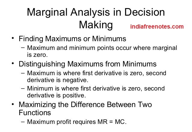
Most of the microeconomic theory of marginalism was developed by Cambridge University professor and economist Alfred Marshall. He stated that production is only beneficial for a firm when marginal revenue exceeds marginal cost, and it is most beneficial when the difference is largest.

For instance, a toy manufacturer should only produce toys until marginal expense is equal to marginal benefit. By breaking down decisions into measurable, smaller pieces, the toy manager can optimize profits.

Marginal analysis has applicability well outside the range of for-profit production processes. Every resource allocation decision can benefit from marginal analysis as long as costs and benefits are identifiable.

Attaining the Highest Net Benefit

Suppose a company is able to measure the additional benefits and costs of extra economic activity. The theory of marginal analysis states that whenever marginal benefit exceeds marginal cost, a manager should increase activity to reach the highest net benefit. Similarly, if marginal cost is higher than marginal benefit, activity should be decreased.

Sunk costs, fixed costs, and average costs do not affect marginal analysis. They are irrelevant to future optimal decision-making. Marginal analysis can only address what happens if the firm hires one additional employee, produces one additional product, devotes additional space to research and so forth.

Marginal Analysis and Opportunity Cost

Managers should also understand the concept of opportunity cost. Suppose a manager knows that there is room in the budget to hire an additional worker. Marginal analysis tells the manager that an additional factory worker provides net marginal benefit. This does not necessarily make the hire the right decision.

Suppose the manager also knows that hiring an additional salesperson yields an even larger net marginal benefit. In this case, hiring a factory worker is the wrong decision because it is sub-optimal.

Market demand is similar to industry demand. It is a broader concept and it involves total demand of a product in an industry. For example, demand of two wheelers in India implies demand of two wheelers produced and marketed by all the companies. It reveals the broader picture of demand. Marketer should keep in mind the wider scenario of industry/market demand to see his position, often called market share of company in an industry. Market demand plays a vital role in formulating the broad marketing programme.

Philip Kotler: “Market demand for the product is the total volume that would be bought by a defined customer group in a defined geographical area in a defined time period in a defined marketing environment under a defined marketing programme.”

Thus, market demand indicates total sales of the product to the specific groups of buyers in a specific period and in defined geographical areas in a given marketing environment.

Elements of Market Demand

Systematic analysis of above stated definitions necessarily reveals following elements:

1. Product

Market demand indicates the total demand of specific products in an industry. The place or scope of product must be specified. In which category or industry the product of company falls. It can be decided on the basis of who are the users and the purpose of using the product. Thus, we must mention the market demand in relation to the specific product.

2. Total Volume

It shows the total volume of sales in form of unit or value. It suggests the total sales of the product in the industry. For example, total volume means the amount (or units) of total demand of refrigerator in India.

3. Purchase or Buying

Only the quantity, that is ordered and purchased is included in market demand. Market demand includes units, which are ordered, delivered, or consumed.

4. Customer Groups

Market demand is expressed in term of different users. Total volume demanded by different groups of customers, such as industrial customers, institutional customers, and individual customers.

5. Geographic Area

Market demand can be specified in term of different geographical areas or localities. It may be in term of country, state, region, district, or any geographic unit.

6. Fixed Time Duration

Market demand is meaningful only if it is expressed in relation to time. For example, demand of two-wheeler during the year 2007. Time may be in term of week, months, quarter, or year.

7. Marketing Environment

Obviously, market demand is influenced by several factors. These factors constitute the marketing environment. So, it is necessary to mention assumptions about marketing environment comprising economic, cultural, social, political, etc., forces.

8. Definition of Marketing Programme

Market demand is affected by marketing programme/strategy. So, it is clarified with reference to a specific marketing programme including product, price, promotion, and distribution. Thus, market demand is stated in context with the definite marketing programme.

While estimating market demand, these all elements should be considered for meaningful picture of total demand. Here, we must distinguish market demand from company demand. Market demand is total demand of the product in an industry, and company demand means demand of the individual business unit’s products. Market forecast relates with market demand and sales forecast relates with company demand. However, market demand forecast and sales forecast are taken loosely (i.e., more or less similar).