Demand theory is a principle relating to the relationship between consumer demand for goods and services and their prices. Demand theory forms the basis for the demand curve, which relates consumer desire to the amount of goods available. As more of a good or service is available, demand drops and so does the equilibrium price.
Demand is the quantity of a good or service that consumers are willing and able to buy at a given price in a given time period. People demand goods and services in an economy to satisfy their wants, such as food, healthcare, clothing, entertainment, shelter, etc. The demand for a product at a certain price reflects the satisfaction that an individual expects from consuming the product. This level of satisfaction is referred to as utility and it differs from consumer to consumer. The demand for a good or service depends on two factors:
- Its utility to satisfy a want or need.
- The consumer’s ability to pay for the good or service. In effect, real demand is when the readiness to satisfy a want is backed up by the individual’s ability and willingness to pay.
Built into demand are factors such as consumer preferences, tastes, choices, etc. Evaluating demand in an economy is, therefore, one of the most important decision-making variables that a business must analyze if it is to survive and grow in a competitive market. The market system is governed by the laws of supply and demand, which determine the prices of goods and services. When supply equals demand, prices are said to be in a state of equilibrium. When demand is higher than supply, prices increase to reflect scarcity. Conversely, when demand is lower than supply, prices fall due to the surplus.
The law of demand introduces an inverse relationship between price and demand for a good or service. It simply states that as the price of a commodity increases, demand decreases, provided other factors remain constant. Also, as the price decreases, demand increases. This relationship can be illustrated graphically using a tool known as the demand curve.
The demand curve has a negative slope as it charts downward from left to right to reflect the inverse relationship between the price of an item and the quantity demanded over a period of time. An expansion or contraction of demand occurs as a result of the income effect or substitution effect. When the price of a commodity falls, an individual can get the same level of satisfaction for less expenditure, provided it’s a normal good. In this case, the consumer can purchase more of the goods on a given budget. This is the income effect. The substitution effect is observed when consumers switch from more costly goods to substitutes that have fallen in price. As more people buy the good with the lower price, demand increases.
Sometimes, consumers buy more or less of a good or service due to factors other than price. This is referred to as a change in demand. A change in demand refers to a shift in the demand curve to the right or left following a change in consumers’ preferences, taste, income, etc. For example, a consumer who receives an income raise at work will have more disposable income to spend on goods in the markets, regardless of whether prices fall, leading to a shift to the right of the demand curve.
The law of demand is violated when dealing with Giffen or inferior goods. Giffen goods are inferior goods that people consume more of as prices rise, and vice versa. Since a Giffen good does not have easily available substitutes, the income effect dominates the substitution effect.
Demand theory is one of the core theories of microeconomics. It aims to answer basic questions about how badly people want things, and how demand is impacted by income levels and satisfaction (utility). Based on the perceived utility of goods and services by consumers, companies adjust the supply available and the prices charged.
Law of Demand
The law of demand is one of the most fundamental concepts in economics. It works with the law of supply to explain how market economies allocate resources and determine the prices of goods and services that we observe in everyday transactions. The law of demand states that quantity purchased varies inversely with price. In other words, the higher the price, the lower the quantity demanded. This occurs because of diminishing marginal utility. That is, consumers use the first units of an economic good they purchase to serve their most urgent needs first, and use each additional unit of the good to serve successively lower valued ends.
- The law of demand is a fundamental principle of economics which states that at a higher price consumers will demand a lower quantity of a good.
- Demand is derived from the law of diminishing marginal utility, the fact that consumers use economic goods to satisfy their most urgent needs first.
- A market demand curve expresses the sum of quantity demanded at each price across all consumers in the market.
- Changes in price can be reflected in movement along a demand curve, but do not by themselves increase or decrease demand.
- The shape and magnitude of demand shifts in response to changes in consumer preferences, incomes, or related economic goods, NOT to changes in price.
Understanding the Law of Demand
Economics involves the study of how people use limited means to satisfy unlimited wants. The law of demand focuses on those unlimited wants. Naturally, people prioritize more urgent wants and needs over less urgent ones in their economic behavior, and this carries over into how people choose among the limited means available to them. For any economic good, the first unit of that good that a consumer gets their hands on will tend to be put to use to satisfy the most urgent need the consumer has that that good can satisfy.
For example, consider a castaway on a desert island who obtains a six pack of bottled, fresh water washed up on shore. The first bottle will be used to satisfy the castaway’s most urgently felt need, most likely drinking water to avoid dying of thirst. The second bottle might be used for bathing to stave off disease, an urgent but less immediate need. The third bottle could be used for a less urgent need such as boiling some fish to have a hot meal, and on down to the last bottle, which the castaway uses for a relatively low priority like watering a small potted plant to keep him company on the island.
In our example, because each additional bottle of water is used for a successively less highly valued want or need by our castaway, we can say that the castaway values each additional bottle less than the one before. Similarly, when consumers purchase goods on the market each additional unit of any given good or service that they buy will be put to a less valued use than the one before, so we can say that they value each additional unit less and less. Because they value each additional unit of the good less, they are willing to pay less for it. So the more units of a good consumers buy, the less they are willing to pay in terms of the price.
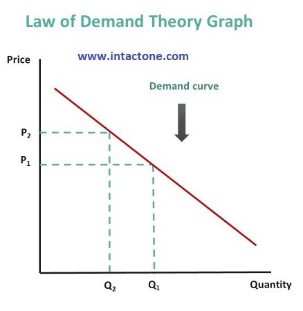
By adding up all the units of a good that consumers are willing to buy at any given price we can describe a market demand curve, which is always downward-sloping, like the one shown in the chart below. Each point on the curve (A, B, C) reflects the quantity demanded (Q) at a given price (P). At point A, for example, the quantity demanded is low (Q1) and the price is high (P1). At higher prices, consumers demand less of the good, and at lower prices, they demand more.
Factors Affecting Demand
The shape and position of the demand curve can be impacted by several factors. Rising incomes tend to increase demand for normal economic goods, as people are willing to spend more. The availability of close substitute products that compete with a given economic good will tend to reduce demand for that good, since they can satisfy the same kinds of consumer wants and needs. Conversely, the availability of closely complementary goods will tend to increase demand for an economic good, because the use of two goods together can be even more valuable to consumers than using them separately, like peanut butter and jelly. Other factors such as future expectations, changes in background environmental conditions, or change in the actual or perceived quality of a good can change the demand curve, because they alter the pattern of consumer preferences for how the good can be used and how urgently it is needed.
Demand theory objectives
- Forecasting sales
- Manipulating demand
- Appraising salesmen’s performance for setting their sales quotas
- Watching the trend of the company’s competitive position.
Of these the first two are most important and the last two are ancillary to the main economic problem of planning for profit.
1. Forecasting Demand
Forecasting refers to predicting the future level of sales on the basis of current and past trends. This is perhaps the most important use of demand studies. True, sales forecast is the foundation for planning all phases of the company’s operations. Therefore, purchasing and capital budget (expenditure) programmes are all based on the sales forecast.
2. Manipulating Demand
Sales forecasting is most passive. Very few companies take full advantage of it as a technique for formulating business plans and policies. However, “management must recognize the degree to which sales are a result only of the external economic environment but also of the action of the company itself.
Sales volumes do differ, “depending upon how much money is spent on advertising, what price policy is adopted, what product improvements are made, how accurately salesmen and sales efforts are matched with potential sales in the various territories, and so forth”.
Often advertising is intended to change consumer tastes in a manner favourable to the advertiser’s product. The efforts of so-called ‘hidden persuaders’ are directed to manipulate people’s ‘true’ wants. Thus sales forecasts should be used for estimating the consequences of other plans for adjusting prices, promotion and/or products.
Importance of Demand Analysis
Demand analysis is vital for forecasting future sales. It helps businesses estimate the quantity of a product that consumers will likely purchase over a specific period. Accurate forecasts enable companies to plan production schedules, manage inventory, allocate resources efficiently, and avoid underproduction or overproduction. This proactive planning improves operational efficiency and reduces costs. Demand forecasting also helps firms adapt to seasonal changes, market trends, and economic fluctuations, ensuring they remain responsive to consumer needs and market conditions.
- Pricing Policy Formulation
Understanding demand is essential for determining the most effective pricing strategy. Through demand analysis, firms can identify how sensitive consumers are to price changes (price elasticity of demand). If demand is inelastic, companies may raise prices without a significant drop in sales. If it is elastic, firms must remain competitive with pricing. Analyzing demand patterns helps in setting optimal prices that balance profitability with consumer satisfaction, ensuring maximum revenue without alienating potential buyers.
- Efficient Resource Allocation
Demand analysis aids in the optimal allocation of limited resources. By knowing which products or services are in high demand, businesses can prioritize investments, labor, and raw materials accordingly. This ensures resources are not wasted on low-demand items. For example, if demand analysis shows growing interest in electric vehicles, manufacturers may divert resources from traditional models to electric production, leading to better financial returns and strategic growth.
- Marketing and Sales Strategy Development
An effective marketing plan depends on a deep understanding of consumer demand. Demand analysis reveals who the buyers are, what they need, and how much they are willing to spend. Businesses can tailor promotions, distribution channels, and product features to match demand patterns. Targeted campaigns and personalized customer engagement strategies become more effective when rooted in accurate demand insights, leading to higher conversion rates and customer loyalty.
- Product Planning and Development
Demand analysis supports product innovation and development decisions. It helps firms identify unmet needs and emerging trends in the market. By studying demand data, companies can decide whether to introduce new products, discontinue existing ones, or modify features to meet changing customer preferences. This reduces the risk of product failure and increases the chances of launching offerings that are relevant, timely, and well-received by consumers.
- Investment Decision-Making
Before investing in new plants, equipment, or market expansion, companies need to assess whether future demand justifies such expenditure. Demand analysis provides the necessary insights to evaluate potential returns on investment. For example, if demand is expected to grow significantly in a region, it may warrant establishing a new facility there. This minimizes financial risk and aligns investment decisions with long-term market opportunities and consumer behavior.
- Helps Government and Policy Makers
Governments and policy makers use demand analysis to make informed decisions about infrastructure, subsidies, taxes, and social welfare programs. By understanding what goods and services are in high demand, governments can align public spending with citizen needs. Demand insights also aid in controlling inflation, managing subsidies, and framing import-export policies. For instance, demand data for housing or healthcare helps governments prioritize urban development and public service improvements.
- Risk Management and Contingency Planning
Demand analysis helps businesses identify potential risks associated with market fluctuations. By studying demand trends, companies can anticipate downturns, supply disruptions, or changing customer preferences. This allows them to develop contingency plans, diversify offerings, or explore new markets in advance. For example, if a drop in demand for fossil fuels is predicted, energy firms can pivot toward renewables. Thus, demand analysis minimizes uncertainty and enhances long-term sustainability.
 by
by