EBIT-EPS analysis for Capital Structure Decision

EBIT-EPS Analysis is a financial tool used to determine the impact of different financing options (debt and equity) on a company’s Earnings Per Share (EPS) at various levels of Earnings Before Interest and Taxes (EBIT). It helps in capital structure decision-making, allowing firms to choose between debt financing (which increases financial leverage) and equity financing (which avoids fixed interest costs but dilutes ownership). The analysis involves computing EPS for different EBIT levels to identify the indifference point, where EPS remains the same regardless of financing choice. Companies aim to maximize EPS while managing financial risk and shareholder value.

Meaning of EBIT

Earnings Before Interest and Taxes (EBIT) refers to the operating profit of the firm.
It is the income earned from business operations before deducting interest on loans and income tax.

EBIT = OperatingRevenue – OperatingExpenses

It measures the earning capacity of the firm independent of financing decisions.

Meaning of EPS

Earnings Per Share (EPS) represents the earnings available to each equity shareholder.
It indicates the profitability of the company from the shareholders’ point of view.

EPS = Earnings available to equity shareholders / Number of equity shares

Higher EPS means higher return to shareholders and increased market value of shares.

Financial Leverage and EBIT–EPS

The analysis is closely related to financial leverage.

Financial leverage means the use of debt in capital structure to increase return to equity shareholders.

  • If EBIT is high → Debt financing increases EPS

  • If EBIT is low → Debt financing decreases EPS

Therefore, proper use of debt can increase shareholders’ wealth.

Advantages of EBIT-EPS Analysis

  • Helps in Selecting Optimum Capital Structure

EBIT–EPS analysis helps management compare different financing alternatives such as equity shares, preference shares and debt. By calculating earnings per share under each plan, the company can identify the most profitable financing option. The plan that provides higher EPS at a particular level of EBIT is selected. Thus, it guides the finance manager in designing an optimum capital structure that balances cost and return while improving the financial performance of the organization.

  • Maximizes Shareholders’ Earnings

The main objective of financial management is to maximize the wealth of equity shareholders. EBIT–EPS analysis directly focuses on earnings available to shareholders. It shows how different financing plans affect EPS and helps management select the alternative that produces higher earnings per share. By choosing the plan with the highest EPS, the firm increases returns to shareholders, enhances investor confidence and improves the market value of shares.

  • Measures the Effect of Financial Leverage

EBIT–EPS analysis clearly explains the effect of financial leverage on shareholders’ earnings. It shows how the use of borrowed funds can increase EPS when operating profits are high. At the same time, it also reveals the negative impact when profits decline. Therefore, it helps management understand both benefits and dangers of debt financing. This knowledge assists in maintaining a proper balance between risk and return while planning the capital structure.

  • Useful in Financial Planning

The analysis is very helpful in financial planning and forecasting. It enables the company to estimate the level of operating profit required to meet interest and dividend obligations. Management can predict future earnings and evaluate the financial viability of proposed financing plans. This makes planning more systematic and reduces uncertainty in financial decision-making. As a result, the company can arrange funds in advance and avoid financial difficulties.

  • Facilitates Comparison of Financing Alternatives

A company often has several alternatives for raising funds, such as issuing shares or taking loans. EBIT–EPS analysis provides a numerical comparison of these alternatives. It presents the impact of each option on EPS in a clear and measurable form. This makes decision-making logical and objective rather than based on assumptions. Hence, management can select the most beneficial financing source after evaluating all possible alternatives.

  • Identifies the Indifference Point

EBIT–EPS analysis helps determine the indifference point, which is the level of EBIT where EPS remains the same under two financing plans. This point guides management in understanding the level of operating income required for debt financing to become advantageous. Above this level, debt financing is preferable, while below it equity financing is safer. Therefore, the indifference point provides a clear basis for selecting suitable financial strategies.

  • Improves Decision-Making

The technique promotes scientific and rational financial decision-making. Instead of relying on guesswork, management uses calculated figures of EPS to choose financing sources. It provides a clear picture of expected returns and financial obligations. This reduces uncertainty and improves confidence in financial decisions. Consequently, the organization can adopt policies that are more effective, practical and aligned with long-term business goals.

  • Assists in Profit Planning

EBIT–EPS analysis also helps in profit planning. By analyzing different EBIT levels, the firm can set profit targets required to achieve desired EPS. Management can evaluate whether expected operating profits are sufficient to cover fixed financial charges. This enables better budgeting and performance evaluation. Therefore, the analysis acts as a useful tool for planning profitability and monitoring the financial performance of the business.

Limitations of EBIT-EPS Analysis


Although EBIT–EPS analysis is a useful technique for selecting an appropriate financing plan and capital structure, it is not free from defects. The analysis mainly concentrates on earnings per share and ignores several practical aspects of financial decision-making. Therefore, it should not be used as the only basis for financing decisions.

The major limitations of EBIT–EPS analysis are explained below:

  • Ignores Business Risk

EBIT–EPS analysis assumes that the operating income (EBIT) is known and stable. In reality, business earnings fluctuate due to changes in demand, competition, economic conditions and technology. If EBIT decreases unexpectedly, the company may not be able to meet interest obligations on debt. Hence, the analysis does not properly consider business risk, which is an important factor in financial planning.

  • Focuses Only on EPS

The technique gives importance only to earnings per share. However, maximizing EPS does not always mean maximizing shareholders’ wealth. Shareholders are also concerned with share price, dividends, safety of investment and future growth. A plan with higher EPS may involve higher risk and may reduce the market value of shares. Therefore, EPS alone is not a complete measure of financial performance.

  • Neglects Financial Risk

EBIT–EPS analysis encourages the use of debt because it often increases EPS at higher levels of EBIT. However, excessive debt increases financial risk and the possibility of insolvency. The company must pay interest regardless of profit. The analysis does not give adequate weight to the risk arising from heavy borrowing, which may endanger the long-term stability of the firm.

  • Assumes Constant Interest and Tax Rates

The analysis assumes that interest rates and tax rates remain constant. In actual business conditions, interest rates change due to market fluctuations and government policies. Similarly, tax rates may also vary. Changes in these rates directly affect EPS and the cost of capital. Hence, results of the analysis may become unrealistic or misleading.

  • Ignores Market Conditions

EBIT–EPS analysis does not consider the condition of the capital market. Sometimes it may not be possible to issue shares or debentures due to unfavorable market situations. Investor preferences, economic recession and stock market trends also affect financing decisions. Since these practical aspects are ignored, the analysis may not always be applicable in real situations.

  • No Consideration of Control

Issue of equity shares reduces the ownership control of existing shareholders. Many companies avoid issuing new shares to maintain management control. EBIT–EPS analysis does not consider this important aspect. It only compares EPS and ignores the effect of financing decisions on voting rights and managerial control.

  • Unrealistic Assumption of Fixed EBIT Levels

The technique compares financing plans at different EBIT levels, but predicting exact EBIT in advance is difficult. Business profits are uncertain and affected by several external factors. If the actual EBIT differs from estimated EBIT, the selected financing plan may not be suitable. Therefore, the analysis may lead to wrong decisions when profit estimates are inaccurate.

  • Does Not Consider Cash Flow Position

EBIT–EPS analysis is based on accounting profits rather than cash flows. However, interest and loan repayments require actual cash payments. A firm may show high EPS but may still face cash shortage. Ignoring liquidity position may create financial difficulties and even bankruptcy.

  • Short-Term Perspective

The analysis mainly focuses on immediate effect on EPS and does not consider long-term consequences such as growth opportunities, financial flexibility and sustainability. A financing plan beneficial in the short run may harm the company in the long run. Therefore, it provides only a partial view of financial decision-making.

Indifference Points:

The indifference point, often called as a breakeven point, is highly important in financial planning because, at EBIT amounts in excess of the EBIT indifference level, the more heavily levered financ­ing plan will generate a higher EPS. On the other hand, at EBIT amounts below the EBIT indifference points the financing plan involving less leverage will generate a higher EPS.

Indifference points refer to the EBIT level at which the EPS is same for two alternative financial plans. According to J. C. Van Home, ‘Indifference point refers to that EBIT level at which EPS remains the same irrespective of debt equity mix’. The management is indifferent in choosing any of the alternative financial plans at this level because all the financial plans are equally desirable. The indifference point is the cut-off level of EBIT below which financial leverage is disadvanta­geous. Beyond the indifference point level of EBIT the benefit of financial leverage with respect to EPS starts operating.

The indifference level of EBIT is significant because the financial planner may decide to take the debt advantage if the expected EBIT crosses this level. Beyond this level of EBIT the firm will be able to magnify the effect of increase in EBIT on the EPS.

In other words, financial leverage will be favorable beyond the indifference level of EBIT and will lead to an increase in the EPS. If the expected EBIT is less than the indifference point then the financial planners will opt for equity for financing projects, because below this level, EPS will be more for less levered firm.

  • Computation:

We have seen that indifference point refers to the level of EBIT at which EPS is the same for two different financial plans. So the level of that EBIT can easily be computed. There are two approaches to calculate indifference point: Mathematical approach and graphical approach.

  • Graphical Approach:

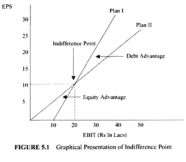
The indifference point may also be obtained using a graphical approach. In Figure 5.1 we have measured EBIT along the horizontal axis and EPS along the vertical axis. Suppose we have two financial plans before us: Financing by equity only and financing by equity and debt. Dif­ferent combinations of EBIT and EPS may be plotted against each plan. Under Plan-I the EPS will be zero when EBIT is nil so it will start from the origin.

The curve depicting Plan I in Figure 5.1 starts from the origin. For Plan-II EBIT will have some positive figure equal to the amount of interest to make EPS zero. So the curve depicting Plan-II in Figure 5.1 will start from the positive intercept of X axis. The two lines intersect at point E where the level of EBIT and EPS both are same under both the financial plans. Point E is the indifference point. The value corresponding to X axis is EBIT and the value corresponding to 7 axis is EPS.

These can be found drawing two perpendiculars from the indifference point—one on X axis and the other on Taxis. Similarly we can obtain the indifference point between any two financial plans having various financing options. The area above the indifference point is the debt advantage zone and the area below the indifference point is equity advantage zone.

Above the indifference point the Plan-II is profitable, i.e. financial leverage is advantageous. Below the indifference point Plan I is advantageous, i.e. financial leverage is not profitable. This can be found by observing Figure 5.1. Above the indifference point EPS will be higher for same level of EBIT for Plan II. Below the indifference point EPS will be higher for same level of EBIT for Plan I. The graphical approach of indifference point gives a better understanding of EBIT-EPS analysis.

Financial Breakeven Point:

In general, the term Breakeven Point (BEP) refers to the point where the total cost line and sales line intersect. It indicates the level of production and sales where there is no profit and no loss because here the contribution just equals to the fixed costs. Similarly financial breakeven point is the level of EBIT at which after paying interest, tax and preference dividend, nothing remains for the equity shareholders.

In other words, financial breakeven point refers to that level of EBIT at which the firm can satisfy all fixed financial charges. EBIT less than this level will result in negative EPS. Therefore EPS is zero at this level of EBIT. Thus financial breakeven point refers to the level of EBIT at which financial profit is nil.

Financial Break Even Point (FBEP) is expressed as ratio with the following equation:

Cost of Debt

Generally, cost of debt capital refers to the total cost or the rate of interest paid by an organization in raising debt capital. However, in a real situation, total interest paid for raising debt capital is not considered as cost of debt because the total interest is treated as an expense and deducted from tax.

This reduces the tax liability of an organization. Therefore, to calculate the cost of debt, the organization needs to make some adjustments. Let us understand the calculation of cost of debt with the help of an example.

Suppose an organization raised debt capital of Rs. 10000 and paid 10% interest on it. The organization is paying corporation tax at the rate of 50%. In this ca.se, the total 10% of interest rate would not be deducted from tax and the deduction would be 50% of 10%.

Therefore, the cost of debt would be only 5%. While calculating cost of debt capital, discount allowed, underwriting commission, and cost of advertisement are also considered. These expenses are added to the amount of interest paid, which is considered as total cost of debt capital.

For example, when an organization increases its proportion of debt capital more than the optimum level, then it increases its risk factor. Therefore, the investors feel insecure and their expectations of EPS start increasing, which is the hidden cost related to debt capital.

Formulae to calculate cost of debt are as follows

  1. When the debt is issued at par

KD = [(1-T)*R]*100

Where,

KD = Cost of debt

T = Tax rate

R = Rate of interest on debt capital

KD = Cost of debt capital

  1. Debt issued at premium or discount when debt is irredeemable

KD = [1/NP*(1-T)* 100]

Where,

NP = Net proceeds of debt

  1. Cost of redeemable debt:

KD = [{I (1-T) -H (P-NP/N) * (1- T)}/ (P -H NP/2)] * 100

Where,

N = Numbers of years of maturity

P = Redeemable value of debt

For example, an organization issued 10% debentures of the face value of Rs. 100 redeemable at par after 20 years.

Assuming 50% tax rate and 5% floatation cost, calculate cost of debt in the following conditions:

  1. When debentures are issued at par
  2. When debentures are issued at 10% discount
  3. When debentures are issued at 10% premium

Solution

The solution is given as follows:

Cost of redeemable debt = [{I (1-T) + (P- NP/N) (1- T)}/ (P + NP/2)] * 100

  1. When debentures are issued at par

KD = [{10(1 – 0.50) + (100 – 95/20) (1 – 0.50)}/ (100 + 95/2)] *100

= 5.25%

  1. When debentures are issued at 10% discount

KD = [{10(1 – 0.50) + (100 – 85/20) (1 – 0.50)}/ (100 + 85/2)] *100

= 5.81%

  1. When debenture is issued at 10% premium

KD = [{10(1 – 0.50) + (100 – 110/20) (1 – 0.50)}/ (100 + 110/2)] *100

= 4.52%

Cost of Preference Shares

Cost of Preference Share Capital: An amount paid by company as dividend to preference shareholder is known as Cost of Preference Share Capital.

Preference share is a small unit of a company’s capital which bears fixed rate of dividend and holder of it gets dividend when company earn profit. Dividend payable is not a tax deductible amount. So, there is no tax adjustments required for comparing with cost of debt.

Formula for Cost of Preference Share:

Irredeemable Preference Share

Redeemable Preference Share

Kp = Dp/NP

Kp = Dp+((RV-NP)/n )/ (RV+NP)/2

Where,

Kp = Cost of Preference Share

Dp = Dividend on preference share

NP = Net proceeds from issue of preference share

(Issue price – Flotation cost)

RV = Redemption Value

N = Period of preference share

Example: A preference share issues at 12% worth Rs 60,000 at 5% discount and after 6 years it redeem at 10% premium. The flotation cost is 5% and tax rate is 20%. Find out the cost of preference share capital.

Solution:

Dividend on preference share (Dp) = 60,000*12/100 = Rs.7200

Discount = 60,000*5/100 = Rs.3000

Flotation Cost = 60,000*5/100 = Rs.3000

Net Proceeds (NP) = Rs. (60,000-3000-3000) = Rs. 54,000

Premium amount = 60,000*10/100 =Rs. 6000

Redemption Value = Rs. (60,000+6000) = Rs. 66,000

Kp = Dp+ ((RV-NP)/n)/ (RV+NP)/2

= 7200+ ((66,000-54,000)/6) / (66,000+54,000)/2

= 9200/60,000

= 15.33%

Cost of Equity Shares

Cost of Equity is the rate of return a company pays out to equity investors. A firm uses cost of equity to assess the relative attractiveness of investments, including both internal projects and external acquisition opportunities. Companies typically use a combination of equity and debt financing, with equity capital being more expensive.

The cost of equity can be calculated by using the CAPM (Capital Asset Pricing Model) or Dividend Capitalization Model (for companies that pay out dividends).

CAPM (Capital Asset Pricing Model)

CAPM takes into account the riskiness of an investment relative to the market. The model is less exact due to the estimates made in the calculation (because it uses historical information).

CAPM Formula:

E(Ri) = Rf + β* [E(Rm) – Rf]

Where:

E(Ri) = Expected return on asset i

Rf = Risk-free rate of return

βi = Beta of asset i

E(Rm) = Expected market return

Risk-Free Rate of Return

The return expected from a risk-free investment (if computing the expected return for a US company, the 10-year Treasury note could be used).

Beta

The measure of systematic risk (the volatility) of the asset relative to the market. Beta can be found online or calculated by using regression: dividing the covariance of the asset and market’s returns by the variance of the market.

βi < 1: Asset i is less volatile (relative to the market)

βi = 1: Asset i’s volatility is the same rate as the market

βi > 1: Asset i is more volatile (relative to the market)

Expected Market Return

This value is typically the average return of the market (which the underlying security is a part of) over a specified period of time (five to ten years is an appropriate range) 

Dividend Capitalization Model

The Dividend Capitalization Model only applies to companies that pay dividends, and it also assumes that the dividends will grow at a constant rate. The model does not account for investment risk to the extent that CAPM does (since CAPM requires beta).

Dividend Capitalization Formula:

Re = (D1 / P0) + g

Where:

Re = Cost of Equity

D1 = Dividends/share next year

P0 = Current share price

g = Dividend growth rate

Dividends/Share Next Year

Companies usually announce dividends far in advance of the distribution. The information can be found in company filings (annual and quarterly reports or through press releases). If the information cannot be located, an assumption can be made (using historical information to dictate whether the next year’s dividend will be similar).

Current Share Price

The share price of a company can be found by searching the ticker or company name on the exchange that the stock is being traded on, or by simply using a credible search engine.

Dividend Growth Rate

The Dividend Growth Rate can be obtained by calculating the growth (each year) of the company’s past dividends and then taking the average of the values.

The growth rate for each year can be found by using the following equation:

Dividend Growth = (Dt/Dt-1) – 1

Where:

Dt = Dividend payment of year t

Dt-1 = Dividend payment of year t-1 (one year before year t)

Cost of Retained Shares

The cost of retained earnings is the cost to a corporation of funds that it has generated internally. If the funds were not retained internally, they would be paid out to investors in the form of dividends. Therefore, the cost of retained earnings approximates the return that investors expect to earn on their equity investment in the company, which can be derived using the capital asset pricing model (CAPM). The CAPM combines the risk-free rate and a stock’s beta to arrive at the cost of equity capital.

Retained Earnings (RE) are the portion of a business’s profits that are not distributed as dividends to shareholders but instead are reserved for reinvestment back into the business. Normally, these funds are used for working capital and fixed asset purchases (capital expenditures) or allotted for paying off debt obligations.

The Purpose of Retained Earnings

Retained earnings represent a useful link between the income statement and the balance sheet, as they are recorded under shareholders’ equity, which connects the two statements. The purpose of retaining these earnings can be varied and includes buying new equipment and machines, spending on research and development, or other activities that could potentially generate growth for the company. This reinvestment into the company aims to achieve even more earnings in the future.

If a company does not believe it can earn a sufficient return on investment from those retained earnings (i.e., earn more than their cost of capital), then they will often distribute those earnings to shareholders as dividends or share buybacks.

Retained Earnings Formula

The RE formula is as follows:

RE = Beginning Period RE + Net Income/Loss – Cash Dividends – Stock Dividends

Where RE = Retained Earnings

Beginning of Period Retained Earnings

At the end of each accounting period, retained earnings are reported on the balance sheet as the accumulated income from the prior year (including the current year’s income), minus dividends paid to shareholders. In the next accounting cycle, the RE ending balance from the previous accounting period will now become the retained earnings beginning balance.

The RE balance may not always be a positive number, as it may reflect that the current period’s net loss is greater than that of the RE beginning balance. Alternatively, a large distribution of dividends that exceed the retained earnings balance can cause it to go negative.

How Net Income Impacts Retained Earnings

Any changes or movement with net income will directly impact the RE balance. Factors such as an increase or decrease in net income and incurrence of net loss will pave the way to either business profitability or deficit. The Retained Earnings account can be negative due to large, cumulative net losses.  Naturally, the same items that affect net income affect RE.

How Dividends Impact Retained Earnings

Distribution of dividends to shareholders can be in the form of cash or stock. Both forms can reduce the value of RE for the business. Cash dividends represent a cash outflow and are recorded as reductions in the cash account. These reduce the size of a company’s balance sheet and asset value as the company no longer owns part of its liquid assets. Stock dividends, however, do not require a cash outflow. Instead, they reallocate a portion of the RE to common stock and additional paid-in capital accounts. This allocation does not impact the overall size of the company’s balance sheet, but it does decrease the value of stocks per share.

End of Period Retained Earnings

At the end of the period, you can calculate your final Retained Earnings balance for the balance sheet by taking the beginning period, adding any net income or net loss, and subtracting any dividends.

Example Calculation

In this example, the amount of dividends paid by XYZ is unknown to us, so using the information from the Balance Sheet and the Income Statement, we can derive it remembering the formula Beginning RE – Ending RE + Net income (-loss) = Dividends

Calculation of Weighted Cost of Capital

Weighted average Cost of Capital (WACC) is a financial metric used to determine the cost of financing a company’s operations. It reflects the average cost of all sources of financing, including debt and equity, weighted by their proportion in the company’s capital structure. The WACC is an important factor in determining a company’s value and profitability, and is used in various financial analysis and decision-making processes.

Components of WACC:

The WACC is composed of two main components:

  • Cost of equity
  • Cost of debt

Cost of Equity:

The cost of equity is the return required by investors in exchange for owning a company’s stock. It reflects the risk associated with owning the stock and is influenced by factors such as market conditions, the company’s financial performance, and the company’s growth prospects. The cost of equity can be calculated using various models, including the dividend discount model, the capital asset pricing model (CAPM), and the arbitrage pricing theory.

Cost of Debt:

The cost of debt is the interest rate paid by a company on its debt financing. It reflects the creditworthiness of the company and market conditions, and is typically lower than the cost of equity. The cost of debt can be calculated using the yield to maturity of the company’s existing debt or by estimating the interest rate the company would have to pay on new debt.

Calculation of WACC:

WACC is calculated by weighting the cost of equity and cost of debt based on their proportion in the company’s capital structure.

WACC = (E/V x Re) + (D/V x Rd x (1 – Tc))

Where:

E = Market value of equity

D = Market value of debt

V = Total market value of the company (E + D)

Re = Cost of equity

Rd = Cost of debt

Tc = Corporate tax rate

The first part of the equation (E/V x Re) represents the cost of equity weighted by the proportion of equity in the company’s capital structure. The second part of the equation (D/V x Rd x (1 – Tc)) represents the cost of debt weighted by the proportion of debt in the company’s capital structure, adjusted for the tax deductibility of interest payments.

Advantages of WACC:

  • Considers all Sources of Financing:

WACC considers the cost of all sources of financing, including debt and equity, which provides a more comprehensive view of the company’s cost of capital.

  • Useful in Decision-making:

WACC is used in various financial analysis and decision-making processes, such as determining whether to undertake a new project or make an acquisition.

  • Reflects Market Conditions:

WACC reflects current market conditions, such as interest rates and the risk premium for equity, which helps companies make informed financial decisions.

  • Easy to Calculate:

WACC is a relatively simple calculation that can be easily understood and communicated to stakeholders.

Limitations of WACC:

  • Assumes constant Capital Structure:

WACC assumes a constant capital structure, which may not be realistic for companies that frequently issue or retire debt or equity.

  • Sensitive to input assumptions:

WACC is sensitive to input assumptions, such as the cost of debt and equity, which can vary depending on the method used to calculate them.

  • Ignores other factors:

WACC does not consider other factors that may affect a company’s cost of capital, such as market risk and company-specific risk.

  • Does not account for Project risk:

WACC is based on the company’s overall risk, and may not accurately reflect the risk associated with a specific project or investment.

Introduction to concept of Leverage

Leverage, as a business term, refers to debt or to borrowing funds to finance the purchase of inventory, equipment and other company assets. Business owners can use either debt or equity to finance or buy the company’s assets. Using debt, or leverage, increases the company’s risk of bankruptcy but, it also can increase the company’s profits and returns; specifically its return on equity. This is true because if debt financing is used rather than equity financing then the owner’s equity is not diluted by issuing more shares of stock.

Borrowing in order to expand or invest is called leverage because the goal is to amplify the loan into a greater value for the firm or investors.

With debt financing, regardless if whether the interest charges are from a loan or line of credit, the interest payments are tax deductible. In addition, by making timely payments a company will establish a positive payment history and business credit rating.

Investors in a business prefer the business to use debt financing but only up to a point. Beyond a certain point, investors get nervous about too much debt financing as it drives up the company’s default risk.

Significance of Leverage

Leverage refers to the use of fixed costs in an attempt to increase the profitability. Leverage affects the level and variability of the firm’s after tax earnings and hence, the firm’s overall risk and return. The study of leverage is significant due to the following reasons.

(i) Measurement of Operating Risk

Operating risk refers to the risk of the firm not being able to cover its fixed operating costs. Since operating leverage depends on fixed operating costs, larger fixed operating costs indicates higher degree of operating leverage and thus, higher operating risk of the firm. High operating leverage is good when sales are rising but bad when they are falling.

(ii) Measurement of Financial Risk

Financial risk refers to the risk of the firm not being able to cover its fixed financial costs. Since financial leverage depends on fixed financial cost, high fixed financial costs indicates higher degree of operating leverage and thus, high financial risk. High financial leverage is good when operating profit is rising and bad when it is falling.

(iii) Managing Risk

Relationship between operating leverage and financial leverage is multiplicative rather than additive. Operating leverage and financial leverage can be combined in a number of different ways to obtain a desirable degree of total leverage and level of total firm risk.

(iv) Designing Appropriate Capital Structure Mix

To design an appropriate capital structure mix or financial plan, the amount of EBIT under various financial plans, should be related to earning per share. One widely used means of examining the effect of leverage to analyze the relationship between EBIT and earning per share.

(v) Increase Profitability

Leverage is an effort or attempt by which a firm tries to show high result or more benefit by using fixed costs assets and fixed return sources of capital. It insures maximum utilization of capital and fixed assets in order to increase the profitability of a firm, It helps to know the reasons not having more profit by a company.

Combined Leverage, Significance, Formula

Combined Leverage refers to the total impact of both operating leverage and financial leverage on a company’s earnings. It measures how changes in sales affect Earnings Per Share (EPS) by considering both fixed operating costs and fixed financial costs (interest on debt). A firm with high combined leverage experiences significant changes in net income when sales fluctuate, making it riskier but potentially more profitable. The Degree of Combined Leverage (DCL) is calculated as the product of the Degree of Operating Leverage (DOL) and the Degree of Financial Leverage (DFL), helping firms assess their overall risk and return potential.

Example:

It should be observed that the leverage is ascertained from a particular sales point. When different levels of sales are adopted, different degrees of composite leverages are obtained. When the volume of sales increases, fixed expenses remains same, the degree of leverage falls. This happens because of existence of fixed charges in the cost structure.

Significance of Combined Leverage

  • Measures Total Risk Exposure

Combined leverage helps assess a company’s overall risk by considering both operating and financial leverage. It indicates the extent to which a firm’s fixed costs (both operational and financial) impact earnings. A higher combined leverage suggests greater sensitivity of Earnings Per Share (EPS) to changes in sales, making it a crucial measure for risk assessment. Companies with high combined leverage must be cautious during economic downturns as small declines in revenue can lead to significant losses, affecting financial stability and investor confidence.

  • Aids in Decision-Making on Capital Structure

Businesses use combined leverage to determine an optimal capital structure by balancing debt and equity. A firm with high operating leverage should maintain low financial leverage to minimize financial risk, whereas firms with low operating leverage may take on more debt. This evaluation helps finance managers decide how much debt financing is suitable while ensuring the firm can cover both operating and financial costs, leading to sustainable growth and profitability.

  • Helps in Profitability Forecasting

By understanding combined leverage, companies can forecast how changes in sales volume will impact their profitability. Since combined leverage magnifies the effect of revenue changes on net income, firms can use this analysis to predict earnings fluctuations and take proactive measures to stabilize cash flows. This is particularly useful for investors and financial analysts in estimating future EPS and making informed investment decisions based on risk and return expectations.

  • Indicates Business Stability and Risk

A firm with high combined leverage is more vulnerable to economic fluctuations, as both high fixed operating costs and high financial obligations increase financial strain. This makes combined leverage an essential indicator of business stability. Companies with lower combined leverage are seen as financially stable since they have more flexibility to manage downturns. Investors and lenders use this measure to assess a company’s ability to withstand economic cycles and make strategic financial decisions accordingly.

  • Assists in Financial Planning

Financial managers use combined leverage to design effective financial strategies that align with the company’s growth objectives. By analyzing leverage levels, businesses can plan for capital expenditures, debt financing, and profit distribution more effectively. A well-balanced leverage structure ensures that firms maximize returns on investment while keeping financial risk at manageable levels. Proper financial planning based on combined leverage helps maintain long-term financial health and stability.

  • Enhances Shareholder Value

Combined leverage plays a crucial role in maximizing shareholder wealth by ensuring a balance between risk and return. A well-structured capital mix enhances earnings per share (EPS) while minimizing financial distress. If managed correctly, combined leverage can lead to higher profitability, attracting more investors and increasing the firm’s market valuation. However, excessive leverage may pose risks, making it essential for firms to maintain a balanced financial structure that supports both growth and stability.

  • Helps in Managing Cost Structure

Businesses must maintain a balance between fixed and variable costs to ensure financial sustainability. Combined leverage helps identify whether a company is relying too much on fixed costs, which could become burdensome during low sales periods. By understanding the proportion of fixed and variable costs, firms can take strategic steps to reduce financial risk, such as renegotiating debt terms, adjusting pricing strategies, or optimizing resource utilization to maintain a competitive edge.

  • Supports Business Expansion Strategies

Companies planning for growth and expansion must carefully evaluate their leverage levels to ensure financial sustainability. High combined leverage can indicate potential constraints on raising additional funds, while lower leverage may signal opportunities for expansion through debt financing. Understanding combined leverage allows businesses to strategically plan expansion without overburdening themselves with excessive debt, ensuring smooth operations and long-term success.

Formula:

Combined leverage considers both financial leverage and operating leverage to assess the overall risk and impact on a company’s earnings. The combined leverage can be calculated using the degree of combined leverage (DCL) or the combined leverage ratio.

  1. Degree of Combined Leverage (DCL):

DCL = DOL × DFL

Where:

  • DOL is the Degree of Operating Leverage.
  • DFL is the Degree of Financial Leverage.

The degree of combined leverage provides a measure of how sensitive a company’s earnings per share (EPS) is to changes in sales.

  1. Combined Leverage Ratio:

Combined Leverage Ratio = % Change in EPS / % Change in Sales​

The combined leverage ratio is another way to express the combined impact of operating and financial leverage on earnings per share.

These formulas help assess how changes in sales can affect a company’s profitability, factoring in both its operating structure (operating leverage) and financing structure (financial leverage). A higher degree of combined leverage means that a company’s earnings are more sensitive to changes in sales, both positively and negatively.

It’s important to note that while leverage can enhance returns, it also introduces additional risk. Therefore, understanding the combined leverage is crucial for effective risk management and financial decision-making. Companies need to strike a balance between leveraging to maximize returns and maintaining financial flexibility to navigate potential challenges.

Operating Leverage, Formula, Uses

Operating Leverage refers to the extent to which a company uses fixed costs in its cost structure to magnify changes in operating profit (EBIT) relative to changes in sales revenue. A firm with high operating leverage has a larger proportion of fixed costs, meaning that a small increase in sales leads to a higher increase in EBIT, but a decline in sales can also result in greater losses. Companies with low operating leverage have more variable costs, making them less risky but with lower profit potential. Measuring Degree of Operating Leverage (DOL) helps in financial planning and risk assessment.

Formula

The operating leverage formula is calculated by multiplying the quantity by the difference between the price and the variable cost per unit divided by the product of quantity multiplied by the difference between the price and the variable cost per unit minus fixed operating costs.

DOL = [Quantity x (Price – Variable Cost per Unit)] / Quantity x (Price – Variable Cost per Unit) – Fixed Operating Costs

By breaking down the equation, you can see that DOL is expressed by the relationship between quantity, price and variable cost per unit to fixed costs. If operating income is sensitive to changes in the pricing structure and sales, the firm is expected to generate a high DOL and vice versa.

You can also rephrase this equation in more general terms like this:

Managers need to monitor DOL to adjust the firm’s pricing structure towards higher sales volumes as a small decrease in sales can lead to a dramatic decrease in profits.

Uses of Operating Leverage:

  • Profit Maximization

Operating leverage helps companies maximize profits by utilizing fixed costs effectively. When sales increase, firms with high operating leverage experience a proportionally larger rise in EBIT (Earnings Before Interest and Taxes), as fixed costs remain constant while revenue grows. This leverage effect allows businesses to enjoy higher profit margins without incurring additional fixed costs. However, firms must carefully manage this leverage since a decline in sales could significantly impact earnings, making profit maximization a delicate balance of cost management and revenue growth strategies.

  • Cost Control and Efficiency

Understanding operating leverage enables firms to focus on cost control and efficiency. Businesses with high fixed costs must ensure that their production processes and operational workflows are optimized to achieve the best possible returns. By closely monitoring cost structures, companies can identify inefficiencies and take corrective actions to improve profitability. This approach also helps in deciding the optimal pricing strategy, ensuring that products are priced competitively while covering fixed costs and generating profits efficiently.

  • Decision-Making in Business Expansion

Operating leverage plays a crucial role in business expansion decisions. Companies with high fixed costs need to evaluate whether increasing production capacity or entering new markets would be financially viable. By analyzing the Degree of Operating Leverage (DOL), firms can predict how additional investments in fixed assets will affect profitability. If an expansion can lead to a significant increase in revenue without proportionally increasing fixed costs, it can be a profitable growth strategy.

  • Risk Assessment and Management

Companies use operating leverage as a tool for risk assessment and management. Businesses with high operating leverage are more sensitive to sales fluctuations, making them riskier in uncertain market conditions. By understanding their leverage position, firms can take measures to mitigate risks, such as diversifying revenue streams, adjusting pricing strategies, or implementing cost-saving measures. A well-managed operating leverage strategy helps in maintaining financial stability during economic downturns.

  • Investment Decision-Making

Investors analyze a company’s operating leverage to assess its profitability potential and financial stability. Firms with high operating leverage offer higher returns when sales increase but also pose greater risks during downturns. Investors evaluate the DOL ratio to determine if a company’s earnings are stable and whether it can generate consistent profits in varying economic conditions. Businesses with a balanced operating leverage approach are often considered safer investment options.

  • Competitive Advantage

Operating leverage helps firms establish a competitive advantage by allowing them to optimize production costs and maintain stable profit margins. Businesses that effectively manage fixed and variable costs can offer competitive pricing while maintaining profitability. This advantage is particularly useful in industries with price-sensitive customers, where companies need to reduce costs while delivering value. A strong operating leverage strategy can help firms outperform competitors and sustain long-term market growth.

  • Budgeting and Financial Planning

Operating leverage is essential in budgeting and financial planning, as it helps businesses forecast profitability under different sales scenarios. Financial managers use operating leverage analysis to prepare budgets that ensure fixed costs are covered even in low-revenue periods. This planning approach helps in making informed decisions regarding cost allocation, production adjustments, and capital investments, ensuring that the company maintains a stable financial position over time.

  • Pricing and Sales Strategy

Companies leverage operating leverage insights to develop effective pricing and sales strategies. High fixed costs require firms to achieve higher sales volumes to break even and generate profits. By understanding their cost structure, businesses can set optimal pricing levels that attract customers while covering operational expenses. Additionally, firms with high operating leverage can implement aggressive marketing and sales strategies to drive revenue growth, ensuring profitability even in competitive markets.

Disability insurance

Disability Insurance, often called DI or disability income insurance, or income protection, is a form of insurance that insures the beneficiary’s earned income against the risk that a disability creates a barrier for a worker to complete the core functions of their work. For example, the worker may suffer from an inability to maintain composure in the case of psychological disorders or an injury, illness or condition that causes physical impairment or incapacity to work. It encompasses paid sick leave, short-term disability benefits (STD), and long-term disability benefits (LTD). Statistics show that in the US a disabling accident occurs, on average, once every second. In fact, nearly 18.5% of Americans are currently living with a disability, and 1 out of every 4 persons in the US workforce will suffer a disabling injury before retirement.

Factors to consider while selecting a disability insurance coverage:

  • Coverage amount: Be diligent in assessing your needs and select the plan, keeping in mind your income level and age. Choose the sum assured such that you and your family could continue to maintain your current lifestyle even if a contingency arises.
  • Determine the disabilities covered: While buying health insurance for disabled, there are a wide variety of options available in the market. Compare the degree of disability (total or partial) and types of disabilities covered across various products and choose the one with the widest coverage.
  • Refund feature: Some products provide the functionality of refund of a part of your premium amount if no claim is made within the specified period.
  • Read the policy wording: For the different degree of disability, different percentages of the sum insured is paid. In the case of partial disability, the percentage may differ depending on the policy wording. So, read the policy document carefully.

There are various government-sponsored health insurance policies for the disabled:

  1. Nirmalya Health Insurance: It is a government-sponsored health insurance scheme for people with mental disabilities. This scheme provides coverage of Rs. 1 Lakh at a low premium rate with benefits including pre and post hospitalisation expenses and OPD treatment.
  2. Swavalamban Health Insurance: It is a custom-tailored insurance scheme to suit the needs of those with disabilities. This plan requires the insured to pay a single premium in one go and avail the coverage at any time of treatment. This policy can be availed only for those disabled individuals with a family income of Rs. 3 Lakh and below. No pre-medical test is required. There is no exclusion of pre-existing conditions. It aims in providing affordable insurance to people with blindness, vision problem, disability related to hearing and mental disabilities.
error: Content is protected !!