Maximization Assignment Problems

There are problems where certain facilities have to be assigned to a number of jobs so as to maximize the overall performance of the assignment. The problem can be converted into a minimization problem in the following ways and then Hungarian method can be used for its solution.

  1. Change the signs of all values given in the table.
  2. Select the highest element in the entire assignment table and subtract all the elements of the table from the highest element.

Example: A marketing manager has five salesmen and sales districts. Considering the capabilities of the salesmen and the nature of districts, the marketing manager estimates that sales per month (in hundred rupees) for each salesman in each district would be as follows. Find the assignment of salesmen to districts that will result in maximum sales.

Maximization Problem

Maximization assignment problem is transformed into minimization problem by

Solution: The given maximization problem is converted into minimization problem by subtracting from the highest sales value (i.e., 41) with all elements of the given table.

Conversion to Minimization Problem

Reduce the matrix row-wise

Matrix Reduced Row-wise

Reduce the matrix column-wise and draw minimum number of lines to cover all the zeros in the matrix, as shown in Table.

Matrix Reduced Column-wise and Zeros Covered

Number of lines drawn ≠ Order of matrix. Hence not optimal.

Select the least uncovered element, i.e., 4 and subtract it from other uncovered elements, add it to the elements at intersection of line and leave the elements that are covered with single line unchanged, Table.

Added & Subtracted the least Uncovered Element

Now, number of lines drawn = Order of matrix, hence optimality is reached. There are two alternative assignments due to presence of zero elements in cells (4, C), (4, D), (5, C) and (5, D).

Two Alternative Assignments

Therefore,

Assignment 1

Assignment 2

Salesman

Districts

Sales (Rs.)

Salesman

Districts

Sales (Rs.)
1 B 38 1 B 38
2 A 40 2 E 36
3 E 37 3 A 41
4 C 41 4 C 41
5 D 35 5 D 35
Total Rs. = 191.00 Total Rs. = 191.00

Unbalanced Assignment Problems

Whenever the cost matrix of an assignment problem is not a square matrix, that is, whenever the number of sources is not equal to the number of destinations, the assignment problem is called an unbalanced assignment problem. In such problems, dummy rows (or columns) are added in the matrix so as to complete it to form a square matrix. The dummy rows or columns will contain all costs elements as zeroes. The Hungarian method may be used to solve the problem.

Example: A company has five machines that are used for four jobs. Each job can be assigned to one and only one machine. The cost of each job on each machine is given in the following Table.

Unbalanced Maximization Assignment problem example

Assignment Problem

Solution: Convert the 4 × 5 matrix into a square matrix by adding a dummy row D5.

Dummy Row D5 Added

Row-wise Reduction of the Matrix

Column-wise reduction is not necessary since all columns contain a single zero. Now, draw minimum number of lines to cover all the zeros, as shown in Table.

All Zeros in the Matrix Covered

Number of lines drawn ≠ Order of matrix. Hence not optimal.

Select the least uncovered element, i.e., 1, subtract it from other uncovered elements, add to the elements at intersection of lines and leave the elements that are covered with single line unchanged as shown in Table.

Subtracted or Added to Elements

Number of lines drawn ≠ Order of matrix. Hence not optimal.

Again Added or Subtracted 1 from Elements

Number of lines drawn = Order of matrix. Hence optimality is reached. Now assign the jobs to machines, as shown in Table.

Assigning Jobs to Machines

Example : In a plant layout, four different machines M1, M2, M3 and M4 are to be erected in a machine shop. There are five vacant areas A, B, C, D and E. Because of limited space, Machine M2 cannot be erected at area C and Machine M4 cannot be erected at area A. The cost of erection of machines is given in the Table.

Assignment Problem

Find the optimal assignment plan.

Solution: As the given matrix is not balanced, add a dummy row D5 with zero cost values. Assign a high cost H for (M2, C) and (M4, A). While selecting the lowest cost element neglect the high cost assigned H, as shown in Table below.

Dummy Row D5 Added

Row-wise reduction of the matrix is shown in Table.

Matrix Reduced Row-wise

Note: Column-wise reduction is not necessary, as each column has at least one single zero. Now, draw minimum number of lines to cover all the zeros, see Table.

Lines Drawn to Cover all Zeros

Number of lines drawn ≠ Order of matrix. Hence not Optimal. Select the smallest uncovered element, in this case 1. Subtract 1 from all other uncovered element and add 1 with the elements at the intersection. The element covered by single line remains unchanged. These changes are shown in Table. Now try to draw minimum number of lines to cover all the zeros.

Added or Subtracted 1 from Elements

Now number of lines drawn = Order of matrix, hence optimality is reached. Optimal assignment of machines to areas are shown in Table.

Optimal Assignment

Hence, the optimal solution is:

Network Analysis

Network technique is a technique for planning, scheduling (programming) and controlling the progress of projects. This is very useful for projects which are complex in nature or where activities are subject to considerable degree of uncertainty in performance time.

This technique provides an effective management, determines the project duration more accurately, identifies the activities which are critical at different stages of project completion to enable to pay more attention on these activities, analyse the scheduling at regular interval for taking corrective action well in advance, facilitates in optimistic resources utilisation, helps management for taking timely and better decisions for effective monitoring and control during execution of the project.

Objectives of Network Analysis:

Network analysis entails a group of techniques for presenting information relating to time and resources so as to assist in the planning, scheduling, and controlling of projects. The infor­mation, usually represented by a network, includes the sequences, interdependencies, interre­lationships, and criticality of various activities of the project.

A network analysis has following objectives:

  1. Powerful tool of planning, scheduling and control.
  2. Shows the inter-relationships of the activities of a project or a programme.
  3. Minimises total cost where the cost of delays and cost of resources required to carry out the tasks can be measured.
  4. Minimise total time where required e.g. in maintenance of production-line machinery in a factory.
  5. Minimization of idle resources.
  6. Minimise production delays.
  7. To provide systematic approach in planning and scheduling.
  8. Follow an integrated approach and bring about better coordination between the de­partments.
  9. Focusses attention on critical activities of the project.
  • Provides up-to-date status information.
  • Suggest areas for increasing efficiency, and reduction of cost.

Applications of Network Technique:

(i) Planning,

(ii) Construction of buildings, bridges, highways, railways, stadiums, irrigation projects, factories, power projects etc.

(iii) Assembly line scheduling,

(iv) Development and launching of new products,

(v) Strategic and tactical military planning,

(vi) Research and development,

(vii) Market penetration programmes,

(viii) Planning of political campaigns,

(ix) Maintenance and overhauling of complicated or large machineries,

(x) organising big conferences etc.

Advantages of Network Technique:

  1. Detailed and thoughtful planning provides better analysis and logical thinking.
  2. Identifies the critical activities and focus them to provide greater managerial atten­tion.
  3. Network technique enables to forecast project duration more accurately.
  4. It is a powerful tool for optimisation of resources by using the concept of slack.
  5. It provides a scientific basis for monitoring, review and control, to evaluate effect of slippages.
  6. It helps in taking decision;

(i) To over-come delays,

(ii) To crashing programme,

(iii) Optimising resources, and

(iv) On other corrective actions.

  1. It helps in getting better co-ordination amongst related fields.
  2. It is an effective management tool through a common and simple language, providing common understanding.

Limitations of Network Techniques:

(i) Network technique is simply a tool to help the management; hence its effectiveness depends on how well it is used by the management.

(ii) Its accuracy depends on the estimation of the data used in the network.

(iii) It is useful only if it is updated regularly and decisions for corrective actions are taken timely.

Programme Evaluation and Review Techniques (PERT)

Program Evaluation and Review Technique (PERT) is a method used to examine the tasked that are in a schedule and determine a variation of the Critical Path Method (CPM). It analyzes the time required to complete each task and its associated dependencies to determine the minimum time to complete a project. It estimates the shortest possible time each activity will take, the most likely length of time, and the longest time that might be taken if the activity takes longer than expected.  

The method was developed by the US Navy in 1957 on the Polaris nuclear submarine project.
To conduct PERT Analysis, three time estimates are obtained (optimistic, pessimistic, and most likely) for every activity along the Critical Path. Then use those estimates in the formula below to calculate how much time for each project stage:

Formula: (P+4M+O)/6

  • Optimistic Time (O): The minimum possible time required to accomplish a task, assuming everything proceeds better than is normally expected.
  • Pessimistic Time (P): The maximum possible time required to accomplish a task, assuming everything goes wrong (excluding major catastrophes).
  • Most likely Time (M): The best estimate of the time required to accomplish a task, assuming everything proceeds as normal.
Task Optimistic (O) Most Likely (M) Pessimistic (P)
Task A 2 4 5
Task B 1 2 3
Task C 2 3 4
Task B 3 5 8
Completion 8 Wks 14 Wks 20 Wks

Example of the three time estimates

Example of a Critical Path Nodal Diagram

PERT Analysis can be conducted using Microsoft Project.

Critical Path Method (CPM)

The Critical Path is the longest path of scheduled activities that must be met in order to execute a project.  This is important for Program Managers (PM) to know since any problems that occur on the critical path can prevent a project from moving forward and be delayed.  Earned Value Management (EVM) analysis focuses on the critical path and near critical paths to identify cost and schedule risks. Other schedule paths might have slack time in them to avoid delaying the entire project unlike the critical path. There might be multiple critical paths on a project.

The Critical Path is determined when analyze a projects schedule or network logic diagram and uses the Critical Path Method (CPM).  The CPM provides a graphical view of the project, predicts the time required for the project, and shows which activities are critical to maintain the schedule.

The seven (7) steps in the CPM are:

  1. List of all activities required to complete the project (see Work Breakdown Structure (WBS)),
  2. Determine the sequence of activities
  3. Draw a network diagram
  4. Determine the time that each activity will take to completion
  5. Determine the dependencies between the activities
  6. Determine the critical path
  7. Update the network diagram as the project progresses

The CPM calculates the longest path of planned activities to the end of the project, and the earliest and latest that each activity can start and finish without making the project longer. This process determines which activities are “critical” (i.e., on the longest path) and which have “total float” (i.e., can be delayed without making the project longer).

The CPM is a project modeling technique developed in the late 1950s by Morgan R. Walker of DuPont and James E. Kelley, Jr. of Remington Rand.

Cost analysis and Crashing the Network

The two important components of any activity are the cost and time. Cost is directly proportional to time and vice versa. For example, in constructing a shopping complex, the expected time of completion can be calculated using be time estimates of various activities. But if the construction has to the finished earlier, it requires additional cost to complete the project. We need to arrive at a time / cost trade-off between total cost of project and total time required to complete it.

Normal time: Normal time is the time required to complete the activity at normal conditions and cost.

Crash time: Crash time is the shortest possible activity time; crashing more than the normal time will increase the direct cost.

Cost Slope in Network Analysis

Cost Slope
Cost slope is the increase in cost per unit of time saved by crashing. A linear cost curve is shown in Figure.

Linear Cost Curve

Cost slope=Crash cost Cc– Normal cost Nc/Normal time Ntt

Example : An activity takes 4 days to complete at a normal cost of Rs. 500.00. If it is possible to complete the activity in 2 days with an additional cost of Rs. 700.00, what is the incremental cost of the activity?

Solution:
Incremental Cost or Cost Slope = Cc– Nc / Ntt
= 700-500/4-2 = Rs. 100.00
It means if one day is reduced we have to spend Rs. 100/- extra per day.

Project Crashing

Procedure for crashing

Step1Draw the network diagram and mark the Normal time and Crash time.

Step2: Calculate TE and TL for all the activities.

Step3Find the critical path and other paths.

Step 4: Find the slope for all activities and rank them in ascending order.

Step 5: Establish a tabular column with required field.

Step 6: Select the lowest ranked activity; check whether it is a critical activity. If so, crash the activity, else go to the next highest ranked activity.

Note: The critical path must remain critical while crashing.

Step 7: Calculate the total cost of project for each crashing.

Step 8: Repeat Step 6 until all the activities in the critical path are fully crashed.

Example: The following Table 8.13 gives the activities of a construction project and other data.

Construction Project Data

If the indirect cost is Rs. 20 per day, crash the activities to find the minimum duration of the project and the project cost associated.

Solution: From the data provided in the table, draw the network diagram and find the critical path.

Network Diagram

From the diagram, we observe that the critical path is 1-2-5 with project duration of 14 days The cost slope for all activities and their rank is calculated as shown in table below

Cost slope=Crash cost Cc– Normal cost Nc/Normal time Ntt

Cost Slope for activity 1– 2 = 80 – 50/6 – 4 = 30/2 = 15.

Cost Slope and Rank Calculated

The available paths of the network are listed down in Table indicating the sequence of crashing.

Sequence of Crashing

Network Diagram Indicating Sequence of Crashing

The sequence of crashing and the total cost involved is given in the following table

Initial direct cost = sum of all normal costs given
= Rs. 490.00

Sequence of Crashing & Total Cost

It is not possible to crash more than 10 days, as all the activities in the critical path are fully crashed. Hence the minimum project duration is 10 days with the total cost of Rs. 970.00.

Decision making under Certainty, Uncertainty, Risk

Decision theory, in statistics, a set of quantitative methods for reaching optimal decisions. A solvable decision problem must be capable of being tightly formulated in terms of initial conditions and choices or courses of action, with their consequences. In general, such consequences are not known with certainty but are expressed as a set of probabilistic outcomes. Each outcome is assigned a “utility” value based on the preferences of the decision maker. An optimal decision, following the logic of the theory, is one that maximizes the expected utility. Thus, the ideal of decision theory is to make choices rational by reducing them to a kind of routine calculation.

Decision-making under Certainty

A condition of certainty exists when the decision-maker knows with reasonable certainty what the alternatives are, what conditions are associated with each alternative, and the outcome of each alternative. Under conditions of certainty, accurate, measurable, and reliable information on which to base decisions is available.

The cause and effect relationships are known and the future is highly predictable under conditions of certainty. Such conditions exist in case of routine and repetitive decisions concerning the day-to-day operations of the business.

Decision-making under Risk:

When a manager lacks perfect information or whenever an information asymmetry exists, risk arises. Under a state of risk, the decision maker has incomplete information about available alternatives but has a good idea of the probability of outcomes for each alternative.

While making decisions under a state of risk, managers must determine the probability associated with each alternative on the basis of the available information and his experience.

Decision-making under Uncertainty:

Most significant decisions made in today’s complex environment are formulated under a state of uncertainty. Conditions of uncertainty exist when the future environment is unpredictable and everything is in a state of flux. The decision-maker is not aware of all available alternatives, the risks associated with each, and the consequences of each alternative or their probabilities.

The manager does not possess complete information about the alternatives and whatever information is available, may not be completely reliable. In the face of such uncertainty, managers need to make certain assumptions about the situation in order to provide a reasonable framework for decision-making. They have to depend upon their judgment and experience for making decisions.

Modern Approaches to Decision-making under Uncertainty:

There are several modern techniques to improve the quality of decision-making under conditions of uncertainty.

The most important among these are:

(1) Risk analysis,

(2) Decision trees and

(3) Preference theory.

Risk Analysis:

Managers who follow this approach analyze the size and nature of the risk involved in choosing a particular course of action.

For instance, while launching a new product, a manager has to carefully analyze each of the following variables the cost of launching the product, its production cost, the capital investment required, the price that can be set for the product, the potential market size and what percent of the total market it will represent.

Risk analysis involves quantitative and qualitative risk assessment, risk management and risk communication and provides managers with a better understanding of the risk and the benefits associated with a proposed course of action. The decision represents a trade-off between the risks and the benefits associated with a particular course of action under conditions of uncertainty.
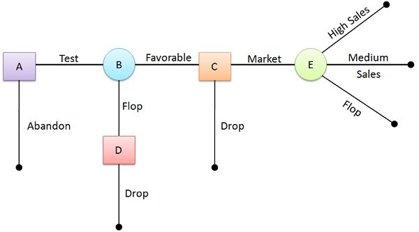
Decision Trees:

These are considered to be one of the best ways to analyze a decision. A decision-tree approach involves a graphic representation of alternative courses of action and the possible outcomes and risks associated with each action.

By means of a “tree” diagram depicting the decision points, chance events and probabilities involved in various courses of action, this technique of decision-making allows the decision-maker to trace the optimum path or course of action.

Preference or Utility Theory:

This is another approach to decision-making under conditions of uncertainty. This approach is based on the notion that individual attitudes towards risk vary. Some individuals are willing to take only smaller risks (“risk averters”), while others are willing to take greater risks (“gamblers”). Statistical probabilities associated with the various courses of action are based on the assumption that decision-makers will follow them.

3For instance, if there were a 60 percent chance of a decision being right, it might seem reasonable that a person would take the risk. This may not be necessarily true as the individual might not wish to take the risk, since the chances of the decision being wrong are 40 percent. The attitudes towards risk vary with events, with people and positions.

Top-level managers usually take the largest amount of risk. However, the same managers who make a decision that risks millions of rupees of the company in a given program with a 75 percent chance of success are not likely to do the same with their own money.

Moreover, a manager willing to take a 75 percent risk in one situation may not be willing to do so in another. Similarly, a top executive might launch an advertising campaign having a 70 percent chance of success but might decide against investing in plant and machinery unless it involves a higher probability of success.

Though personal attitudes towards risk vary, two things are certain.

Firstly, attitudes towards risk vary with situations, i.e. some people are risk averters in some situations and gamblers in others.

Secondly, some people have a high aversion to risk, while others have a low aversion.

Most managers prefer to be risk averters to a certain extent, and may thus also forego opportunities. When the stakes are high, most managers tend to be risk averters; when the stakes are small, they tend to be gambler.

Decision Tree Analysis

Decision Tree may be understood as the logical tree, is a range of conditions (premises) and actions (conclusions), which are depicted as nodes and the branches of the tree which link the premises with conclusions. It is a decision support tool, having a tree-like representation of decisions and the consequences thereof. It uses ‘AND’ and ‘OR’ operators, to recreate the structure of if-then rules.

A decision tree is helpful in reaching the ideal decision for intricate processes, especially when the decision problems are interconnected and chronological in nature.

decision tree does not constitute a decision but assists in making one, by graphically representing the material information related to the given problem, in the form of a tree. It diagrammatically depicts various courses of action, likely outcomes, states of nature, etc. as nodes, branches or sub-branches of a horizontal tree.

Nodes

There are two types of Nodes:

  • Decision Node: Represented as square, wherein different courses of action arise from decision node in main branches.
  • Chance Node: Symbolised as a circle, at the terminal point of decision node, the chance node is present, where they emerge as sub-branches. These depict probabilities and outcomes.

For instance: Think of a situation where a firm introduces a new product. The decision tree presented below gives a clear idea of managerial problems.

  • Key A is a decision node, wherein the decision is taken, i.e. to test the product or drop the same.
  • Key B is an outcome node, which shows all possible outcomes, that can be taken. As per the given situation, there are only two outcomes, i.e. favorable or not.
  • Key C is again a decision node, that describes the market test is positive, so the firm’s management will decide whether to go further with complete marketing or drop the product.
  • Key D is one more decision node, but does not shows any choice, which depicts that if the market test is unfavorable then the decision is to drop the product.
  • Key E is again an outcome node.

The decision tree can be applied to various areas, where decisions are pending such as make or buy decision, investment decision, marketing strategy, the introduction of a new project. The decision maker will go for the alternative that increases the anticipated profit or the one which reduces the overall expected cost at each decision point.

Types of Decision Tree

In a single stage decision tree, the decision maker can find only one solution, which is the best course of action, on the basis of the information gathered. On the other hand, multi-stage decision tree involves a series of the decision to be taken.

Decision Tree Analysis

The Decision Tree Analysis is a schematic representation of several decisions followed by different chances of the occurrence. Simply, a tree-shaped graphical representation of decisions related to the investments and the chance points that help to investigate the possible outcomes is called as a decision tree analysis.

The decision tree shows Decision Points, represented by squares, are the alternative actions along with the investment outlays, that can be undertaken for the experimentation. These decisions are followed by the chance points, represented by circles, are the uncertain points, where the outcomes are dependent on the chance process. Thus, the probability of occurrence is assigned to each chance point.

Once the decision tree is described precisely, and the data about outcomes along with their probabilities is gathered, the decision alternatives can be evaluated as follows:

  1. Start from the extreme right-hand end of the tree and start calculating NPV for each chance points as you proceed leftward.
  2. Once the NPVs are calculated for each chance point, evaluate the alternatives at the final stage decision points in terms of their NPV.
  3. Select the alternative which has the highest NPV and cut the branch of inferior decision alternative. Assign value to each decision point equivalent to the NPV of the alternative selected.
  4. Again, repeat the process, proceed leftward, recalculate NPV for each chance point, select the decision alternative which has the highest NPV value and then cut the branch of the inferior decision alternative. Assign the value to each point equivalent to the NPV of selected alternative and repeat this process again and again until a final decision point is reached.

Thus, decision tree analysis helps the decision maker to take all the possible outcomes into the consideration before reaching a final investment decision.

decision tree is a decision support tool that uses a tree-like model of decisions and their possible consequences, including chance event outcomes, resource costs, and utility. It is one way to display an algorithm that only contains conditional control statements.

Decision trees are commonly used in operations research, specifically in decision analysis, to help identify a strategy most likely to reach a goal, but are also a popular tool in machine learning.

Linear Programming

The technique of linear programming was formulated by a Russian mathematician L.V. Kantorovich. But the present version of simplex method was developed by Geoge B. Dentzig in 1947. Linear programming (LP) is an important technique of operations research developed for optimum utilization of resources.

It is an important optimization (maximization or minimization) technique used in decision making is business and everyday life for obtaining the maximum or minimum values as required of a linear expression to satisfying certain number of given linear restrictions.

Common terminologies used in Linear Programming

  • Decision Variables: The decision variables are the variables which will decide my output. They represent my ultimate solution. To solve any problem, we first need to identify the decision variables. For the above example, the total number of units for A and B denoted by X & Y respectively are my decision variables.
  • Objective Function: It is defined as the objective of making decisions. In the above example, the company wishes to increase the total profit represented by Z. So, profit is my objective function.
  • Constraints: The constraints are the restrictions or limitations on the decision variables. They usually limit the value of the decision variables. In the above example, the limit on the availability of resources Milk and Choco are my constraints.
  • Non-negativity restriction: For all linear programs, the decision variables should always take non-negative values. Which means the values for decision variables should be greater than or equal to 0.

Characteristics:

(a) Objective function:

There must be clearly defined objec­tive which can be stated in quantitative way. In business problems the objective is generally profit maximization or cost minimization.

(b) Constraints:

All constraints (limitations) regarding resources should be fully spelt out in mathematical form.

(c) Non-negativity:

The value of variables must be zero or positive and not negative. For example, in the case of production, the manager can decide about any particular product number in positive or minimum zero, not the negative.

(d) Linearity:

The relationships between variables must be linear. Linear means proportional relationship between two ‘or more variable, i.e., the degree of variables should be maximum one.

(e) Finiteness:

The number of inputs and outputs need to be finite. In the case of infinite factors, to compute feasible solution is not possible.

Advantages of Linear Programming

  1. LP makes logical thinking and provides better insight into business problems.
  2. Manager can select the best solution with the help of LP by evaluating the cost and profit of various alternatives.
  3. LP provides an information base for optimum alloca­tion of scarce resources.
  4. LP assists in making adjustments according to changing conditions.
  5. LP helps in solving multi-dimensional problems.

Assumptions:

(i) There are a number of constraints or restrictions- expressible in quantitative terms.

(ii) The prices of input and output both are constant.

(iii) The relationship between objective function and constraints are linear.

(iv) The objective function is to be optimized i.e., profit maximization or cost minimization.

Application Area

In business, executives need to make a plethora of decisions. From which company will provide and stock the break room’s vending machines to which costs get cut during a lean time, all require careful thought and planning. It’s essential that every decision, no matter what its perceived importance may be, be made with the best intentions and the company’s best interests at heart.

The Health of the Business Depends on It: Making snap business decisions can make or break a business. Changing business practices on a whim or because an owner is in a bad mood can have irreversible consequences. All business decisions should be carefully considered, and should preferably have input from several others. The business owner has the final say, but other voices should be brought to the table so that all sides of an issue can be considered.

It Takes a Team: A business is only as good as its weakest member, so putting together a strong management group is paramount to the business’ ability to make good decisions, which leads to the success of the business. All members of management need to be on the same page, as to what constitutes the mission and objectives of the business. Once everybody knows the mission, deciding how to meet its objectives becomes easier. If you value a person enough to put her on the team, then you should value that person’s opinion, even if it disagrees with yours.

Consult Someone With More Expertise: If you don’t feel secure enough in your abilities or in your team’s abilities to make a solid decision, there is nothing wrong with getting help from someone outside of the company. For example, a graphics design firm might consult with an attorney to look over a new contract, or an attorney might hire an accountant to assist with the financial statements for the law firm. No one is an expert at everything, and good decision making includes knowing when to seek additional assistance.

Don’t Be Afraid to Reverse: Sometimes, a decision made needs to be revisited. A business move that was ideal in January might not be as effective in July. Evaluating previous business decisions and choosing to modify or completely reverse that decision is acceptable. Although long-term, permanent decisions are typically the goal, sometimes, you have to think short-term and then revisit the issue at a later date.

Gray Areas: Not every decision is black and white. In some cases, you have to look at the gray area, as well. This is where having a strong management team or additional expertise comes into play. These people can help a business owner see all sides of an issue, which improves the chances of making a keen business decision that’s in the company’s best interest.

Graphical Solutions of LLP

Owing to the importance of linear programming models in various industries, many types of algorithms have been developed over the years to solve them. Some famous mentions include the Simplex method, the Hungarian approach, and others. Here we are going to concentrate on one of the most basic methods to handle a linear programming problem i.e. the graphical method.

In principle, this method works for almost all different types of problems but gets more and more difficult to solve when the number of decision variables and the constraints increases.

We will first discuss the steps of the algorithm:

Step 1: Formulate the LP (Linear programming) problem

We have already understood the mathematical formulation of an LP problem in a previous section. Note that this is the most crucial step as all the subsequent steps depend on our analysis here.

Step 2: Construct a graph and plot the constraint lines

The graph must be constructed in ‘n’ dimensions, where ‘n’ is the number of decision variables. This should give you an idea about the complexity of this step if the number of decision variables increases.

One must know that one cannot imagine more than 3-dimensions anyway! The constraint lines can be constructed by joining the horizontal and vertical intercepts found from each constraint equation.

Step 3: Determine the valid side of each constraint line

This is used to determine the domain of the available space, which can result in a feasible solution. How to check? A simple method is to put the coordinates of the origin (0,0) in the problem and determine whether the objective function takes on a physical solution or not. If yes, then the side of the constraint lines on which the origin lies is the valid side. Otherwise it lies on the opposite one.

Step 4: Identify the feasible solution region

The feasible solution region on the graph is the one which is satisfied by all the constraints. It could be viewed as the intersection of the valid regions of each constraint line as well. Choosing any point in this area would result in a valid solution for our objective function.

Step 5: Plot the objective function on the graph

It will clearly be a straight line since we are dealing with linear equations here. One must be sure to draw it differently from the constraint lines to avoid confusion. Choose the constant value in the equation of the objective function randomly, just to make it clearly distinguishable.

Step 6: Find the optimum point

Optimum Points

An optimum point always lies on one of the corners of the feasible region. How to find it? Place a ruler on the graph sheet, parallel to the objective function. Be sure to keep the orientation of this ruler fixed in space. We only need the direction of the straight line of the objective function. Now begin from the far corner of the graph and tend to slide it towards the origin.

  • If the goal is to minimize the objective function, find the point of contact of the ruler with the feasible region, which is the closest to the origin. This is the optimum point for minimizing the function.
  • If the goal is to maximize the objective function, find the point of contact of the ruler with the feasible region, which is the farthest from the origin. This is the optimum point for maximizing the function.

Step 7: Calculate the coordinates of the optimum point.

This is the last step of the process. Once you locate the optimum point, you’ll need to find its coordinates. This can be done by drawing two perpendicular lines from the point onto the coordinate axes and noting down the coordinates.

Otherwise, you may proceed algebraically also if the optimum point is at the intersection of two constraint lines and find it by solving a set of simultaneous linear equations. The Optimum Point gives you the values of the decision variables necessary to optimize the objective function.

The Graphical Method (graphic solving) is an excellent alternative for the representation and solving of Linear Programming models that have two decision variables.

Exercise #1: A workshop has three (3) types of machines A, B and C; it can manufacture two (2) products 1 and 2, and all products have to go to each machine and each one goes in the same order; First to the machine A, then to B and then to C. The following table shows:

  • The hours needed at each machine, per product unit
  • The total available hours for each machine, per week
  • The profit of each product per unit sold
Type of Machine Product 1 Product 2 Available hours per week
A 2 2 16
B 1 2 12
C 4 2 28
Profit per Unit 1 1.50  

Formulate and solve using the graphical method a Linear Programming model for the previous situation that allows the workshop to obtain maximum gains.

Decision Variables:

  • : Product 1 Units to be produced weekly
  • : Product 2 Units to be produced weekly

Objective Function:

Maximize2 

Constraints:

The constraints represent the number of hours available weekly for machines A, B and C, respectively, and also incorporate the non-negativity conditions.

For the graphical solution of this model we will use the Graphic Linear Optimizer (GLP) software. The green colored area corresponds to the set of feasible solutions and the level curve of the objective function that passes by the optimal vertex is shown with a red dotted line.

The optimal solution is  and  with an optimal value  that represents the workshop’s profit.

error: Content is protected !!