Year: 2020

Advantages of Simulation

Simulation offers various advantages. They have applications in every field. But this article covers the advantages of simulation in mechanical design only.

System Behavior Analysis

Simulations are used to analyze the behavior of a system without actually building it. Engineers can work on alternative solutions and simulate various designs. Therefore advantages of simulation include finalizing the best solution for prototyping before actually building it.

Reduces Manufacturing Cost

Simulation offers the advantage of designing products first time right. Therefore manufacturing and testing costs are reduced significantly.

Faster Products to Market

Advantages of Simulation studies include reduced number of design iterations. Therefore Design cycle time reduces significantly. This gives companies advantage of launching products in the market faster.

Design Analysis: Visual Output

Simulation results can be exported in graphical representation. It helps in analyzing system and product performance.

Problem Solving

Simulations are used to analyze a problem at various levels. This leads to faster and effective problem solving.

Value Engineering

Simulation studies helps in reducing manufacturing cost of existing and new products. For example mold-flow analysis is used to reduce injection molding cycle time.

Disadvantages of Simulation studies

Along with so many advantages, simulation studies also have some disadvantages. But the fact is overall simulation studies are good for a design.

Higher Initial Investment

Disadvantages of simulation software involve high initial investment. Such as high software cost and computing power requirements. Therefore small companies can not afford them.

Accurate Boundary conditions and input Data

Simulation results accuracy depends on input data and boundary conditions. System boundary conditions include environmental temperature, pressure and material.

Therefore boundary conditions need to be defined accurately to achieve good results. It requires a lot of experience.

Not 100% Accurate

Simulation softwares are not 100% accurate. You should expect some discrepancies in simulation results and tested products. With time engineers can refine their simulation results.

Main advantages of simulation include:

• Study the behavior of a system without building it.
• Results are accurate in general, compared to analytical model.
• Help to find un-expected phenomenon, behavior of the system.
• Easy to perform “What-If” analysis.

Main disadvantages of simulation include:

• Expensive to build a simulation model.
• Expensive to conduct simulation.
• Sometimes it is difficult to interpret the simulation results.

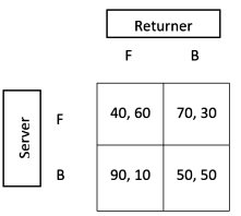
The simplest model is a duopoly market in which each duopolist attempts to maximise his market share.

Given this goal, whatever a firm gains (by increasing its share of the market) the other firm loses (because of the decrease in its share).

Thus any gain of one rival is offset by the loss of the other, and the net gain sums up to zero. Hence the name ‘zero-sum game’.

The assumptions of the model are:

1. The firms have a given, well-defined goal. In our particular example the goal is maximisation of the market share.
2. Each firm knows the strategies open to it and to its rival, or concentrates on the most important of these strategies.
3. Each firm knows with certainty the payoffs of all combinations of the strategies being considered. This implies that the firm knows its total revenue, total costs and total profit from each combination of strategies.
4. The actions chosen by the duopolists do not affect the total size of the market.
5. Each firm chooses its strategy ‘expecting the worst from its rival’, that is, each firm acts in the most conservative way, expecting that the rival will choose the best possible counter-strategy open to him. This behaviour is defined as ‘rational’.
6. In the zero-sum game there is no incentive for collusion, given assumption 4, since the goals of the firms are diametrically opposed.

In order to find the equilibrium solution we need information on the payoff matrix of the two firms. In our example the payoffs will be shares of the market resulting from the adoption of any two strategies by the rivals. Assume that Firm I has four strategies open to it and Firm II has five strategies. The payoff matrices of the duopolists are shown in tables 19.2 and 19.3.

Clearly the sum of the payoffs in corresponding cells of the two payoff tables adds up to unity, since the numbers in these cells are shares, and the total market is shared between the two firms. In general, in the two-person zero-sum game we need not write both payoff matrices because of the nature of the game: the goals are opposing, and, in our example, the payoff table of Firm I contains indirectly information about the pay­off of Firm II. Still we start by showing both tables, and then we show how the equi­librium solution can be found from only the first payoff matrix.

Choice of strategy by Firm I:

Firm I examines the outcomes of each strategy open to it. That is, Firm I examines each row of its payoff matrix and finds the most favourable outcome of the corres­ponding strategy, because the firm expects the rival to adopt the most advantageous action open to him. This is the behavioural rule implied by assumption 5 of this model.

Thus:

If Firm I adopts strategy A₁, the worst outcome that it may expect is a share of 0.10 (which will be realized if the rival Firm II adopts its most favourable strategy B₁).

If Firm I adopts strategy A₂, the worst outcome will be a share of 0.30 (if the rival adopts the best action for him, B₂).

If Firm I adopts strategy A₃, the worst outcome will be a share of 0.20 (if Firm II chooses the best open alternative, B₃).

If Firm I adopts strategy A₄, the worst outcome will be a share of 0.15 (which would be realised by action B₂ of Firm II).

Among all these minima (that is, among the above worst outcomes) Firm I chooses the maximum, the ‘best of the worst’. This is called a maximin strategy, because the firm chooses the maximum among the minima. In our example the maximin strategy of Firm I is A₂, that is, the strategy which yields a share of 0.30.

Choice of strategy by Firm II:

Firm II behaves in exactly the same way. The only difference is that Firm II examines the columns of its payoff table, because these columns include the results-payoffs of each of the strategies open to Firm II. For each strategy, that is, for each column, Firm II finds the worst outcome (on the assumption that the rival will choose the best), and among these worst outcomes Firm II chooses the best. Thus, if Firm II uses its own payoff table, its behaviour is a maximin behaviour identical to the behaviour of Firm I.

However, in the zero-sum game only one payoff matrix is adequate for the equilibrium solution. In our example the first payoff table will be used not only by Firm I but also by Firm II. Thus concentrating on the first payoff table we may re­state the decision-making process of Firm II as follows. Firm II examines the columns of the (first) payoff matrix because these columns contain the information about the payoffs of its strategies.

For each column-strategy Firm II finds the maximum payoff (of Firm I) because this is the worst situation the firm (II) will face if it adopts the strategy corresponding to that column. Thus for strategy B_{ the worst outcome (for Firm II) is 0-40; for strategy B₂ the worst outcome is 0-30; for strategy B₃ the worst outcome is 0-50; for strategy fl₄ the worst result is 0-60; for strategy B_s the worst result is 0-50. Among these maxima of each column-strategy Firm II will choose the strategy with minimum value. Thus the strategy of Firm II is a minimax strategy, since it involves the choice of a minimum among the maxima payoffs. (Table 19.4.)

It should be stressed that although different terms are used for the choice of the two firms (maximin behaviour of Firm I, minimax behaviour of Firm II), the behavioural rule for both firms is the same: each firm expects the worst from its rival.

In our example the equilibrium solution is strategy A₂ for Firm I and B₂ for Firm II. This solution yields shares 0 30 for Firm I and 0-70 for Firm II. It is an equilibrium solution because it is the preferred one by both firms. This solution is called the ‘saddle point’, and the preferred strategies A₂ and B₂ are called ‘dominant strategies’.

It should be clear that there exists no such equilibrium (saddle) solution if there is no payoff which is preferred by both firms simultaneously. Under certain mathematical conditions other solutions and strategy choices can be determined. The analysis of the resulting mixed strategies requires a sophisticated exposition of utility theory and random selection which is beyond the scope of this book.

1. Uncertainty Model:

The assumption that each firm knows with certainty the exact value of the payoff of each strategy is unrealistic. The most probable situation in the real business world is that the firm, by adopting a certain strategy, may expect a range of results for each counter-strategy of the rival, each result with an associated probability. Thus the payoff matrix is constructed so as to include the expected value of each payoff.

The expected value is the sum of the products of the possible outcomes of a pair of strategies (adopted by the two firms) each multiplied by its probability:

where g_si = the sth of the n possible outcomes of strategy i of Firm I (given that Firm II has chosen strategy j)

P_S = the probability of the sth outcome of strategy i

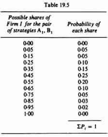
For example, assume that Firm I chooses strategy A₁ and Firm II reacts with strategy B₁. This pair of simultaneous strategies may yield the shares for Firm I each with a certain probability, shown in the second column of table 19.5. Thus the expected payoff of the pair of strategies A₁ and B₁ is

E(G_{1 1}) = (0.00)(0.00) + (0.05) (0.05) + (0.15)(0.05) + … + (0.95)(0.02) + (1)(0) = 0.458

In a similar way we find the expected payoff of all combinations of strategies. Given the matrix of expected payoffs, the behavioural pattern of the firms is the same as in the certainty model.

That is:

Firm I adopts the maximin strategy. It finds for each row the minimum expected payoff, and among these minima the firm chooses the one with the highest value (the maximum among the minima).

Firm II adopts the minimax strategy. It finds for each column the maximum expected payoff, and among these maxima Firm II chooses the one with the smallest value (the minimum among the maxima).

Although the uncertainty zero-sum game seems simple, its assumptions are quite stringent:

1. The firms maximise their expected payoffs.
2. The zero-sum game assumes that both firms assign the same probability to each pair of payoffs; they make the same judgement. This implies that the firms must have the same information and the same objective criteria with which to evaluate the probabilities of the different payoffs. Otherwise the probability distribution of the payoffs will not be objective.
3. The firms maximise their total utility, and the utility of each payoff is proportional to the value assumed by the payoff.

The above assumptions are clearly strong and unrealistic. Furthermore, the basic condition of the zero-sum game that the ‘gain’ of one firm is equal to the ‘loss’ of the other, is rarely met in the real business world. Usually the ‘gains’ are not ‘offset’ by equal ‘losses’. Only in the case of a share goal, and in the rare case of extinction tactics, do we have a zero-sum game. In most cases we have a non-zero-sum game.

Pure strategy

A pure strategy is an unconditional, defined choice that a person makes in a situation or game. For example, in the game of Rock-Paper-Scissors,if a player would choose to only play scissors for each and every independent trial, regardless of the other player’s strategy, choosing scissors would be the player’s pure strategy. The probability for choosing scissors equal to 1 and all other options (paper and rock) is chosen with the probability of 0. The set of all options (i.e. rock, paper, and scissors) available in this game is known as the strategy set.

Mixed strategy

A mixed strategy is an assignment of probability to all choices in the strategy set. Using the example of Rock-Paper-Scissors, if a person’s probability of employing each pure strategy is equal, then the probability distribution of the strategy set would be 1/3 for each option, or approximately 33%. In other words, a person using a mixed strategy incorporates more than one pure strategy into a game.

The definition of a mixed strategy does not rule out the possibility for an option(s)to never be chosen (eg. p_scissors= 0.5, p_rock = 0.5, p_paper = 0). This means that in a way, a pure strategy can also be considered a mixed strategy at its extreme, with a binary probability assignment (setting one option to 1 and all others equal to 0). For this article, we shall say that pure strategies are not mixed strategies.

In the game of tennis, each point is a zero-sum game with two players (one being the server S, and the other being the returner R). In this scenario, assume each player has two strategies (forehand F, and backhand B). Observe the following hypothetical in the payoff matrix:

The strategies F_S or B_S are observed for the server when the ball is served to the side of the service box closest to the returner’s forehand or backhand, respectively. For the returner, the strategies F_R and B_R are observed when the returner moves to the forehand or backhand side to return the serve, respectively. This gives us the payoffs when the returner receives the serve correctly (F_S,F_R or B_S,B_R), or incorrectly (F_S,B_R or B_S,F_R). The payoffs to each player for every action are given in pure strategy payoffs, as each player is only guaranteed their payoff given the opponent’s strategy is employed 100% of the time. Given these pure strategy payoffs, we can calculate the mixed strategy payoffs by figuring out the probability each strategy is chosen by each player.

So you are Roger. It is apparent to you that a pure strategy would be exploitable. If you serve to the backhand 100% of the time, it would be easy for the opponent to catch on and return from the backhand side more often than the forehand, maximizing his expected payoff. Same goes for the serve to the forehand. But how often should you mix your strategy and serve to each side to minimize your opponent’s chances of winning? Calculating these probabilities would give us our mixed strategy Nash equilibria, or the probabilities that each strategy is used which would minimize the opponent’s expected payoff. In the following article, we will look at how to find mixed strategy Nash equilibria, and how to interpret them.

Pure and Mixed Strategies:

In a pure strategy, players adopt a strategy that provides the best payoffs. In other words, a pure strategy is the one that provides maximum profit or the best outcome to players. Therefore, it is regarded as the best strategy for every player of the game. In the previously cited example (Table-1), the increase in the prices of organizations’ products is the best strategy for both of them.

This is because if both of them increase the prices of their products, they would earn maximum profits. However, if only one of the organization increases the prices of its products, then it would incur losses. In such a case, an increase in prices is regarded as a pure strategy for organizations ABC and XYZ.

On the other hand, in a mixed strategy, players adopt different strategies to get the possible outcome. For example, in cricket a bowler cannot throw the same type of ball every time because it makes the batsman aware about the type of ball. In such a case, the batsman may make more runs.

However, if the bowler throws the ball differently every time, then it may make the batsman puzzled about the type of ball, he would be getting the next time.

Therefore, strategies adopted by the bowler and the batsman would be mixed strategies, which are shown ion Table2:

In Table-2, when the batsman’s expectation and the bowler’s ball type are same, then the percentage of making runs by batsman would be 30%. However, when the expectation of the batsman is different from the type of ball he gets, the percentage of making runs would reduce to 10%. In case, the bowler or the batsman uses a pure strategy, then any one of them may suffer a loss.

Therefore, it is preferred that bowler or batsman should adopt a mixed strategy in this case. For example, the bowler throws a spin ball and fastball with a 50-50 combination and the batsman predicts the 50-50 combination of the spin and fast ball. In such a case, the average hit of runs by batsman would be equal to 20%.

This is because all the four payoffs become 25% and the average of four combinations can be derived as follows:

0.25(30%) + 0.25(10%) + 0.25(30%) + 0.25(10%) = 20%

However, it may be possible that when the bowler is throwing a 50-50 combination of spin ball and fastball, the batsman may not be able to predict the right type of ball every time. This would decrease his average run rate below 20%. Similarly, if the bowler throws the ball with a 60-40 combination of fast and spin ball respectively, and the batsman would expect either a fastball or a spin ball randomly. In such a case, the average of the batsman hits remains 20%.

The probabilities of four outcomes now become:

Anticipated fastball and fastball thrown: 0.50*0.60 = 0.30

Anticipated fastball and spin ball thrown: 0.50*0.40 = 0.20

Anticipated spin ball and spin ball thrown: 0.50*0.60 = 0.30

Anticipated spin ball and fastball thrown: 0.50*0.40 = 0.20

When we multiply the probabilities with the payoffs given in Table-2, we get

0.30(30%) + 0.20(10%) + 0.20(30%) + 0.30(10%) = 20%

This shows that the outcome does not depends on the combination of fastball and spin ball, but it depends on the prediction of the batsman that he can get any type of ball from the bowler.

Queuing theory is the study of queues and the random processes that characterize them. It deals with making mathematical sense of real-life scenarios. For example, a mob of people queuing up at a bank or the tasks queuing up on your computer’s back end.

In queuing theory we often want to find out how long wait times or queue lengths are, and we can use models to do this. These models are typically important in business and software applications, and queueing theory is often considered a part of operations research.

About Queuing

Any queuing activity can be summarized as entities (customers in your supermarket queue, or jobs in a computer queue) trying to get through an activity (waiting to be served). Queues happen when we can’t all access the activity at the same time: when it is not economically efficient to have enough checkout lines for everyone to go right through as soon as they were ready, or there isn’t enough server space to do an unlimited amount of computer tasks at one moment.

In queueing theory a queue does not refer simply to a neat row which is always first come, first served. This is one example of a queue, but not the only kind. A mob trying to rush for the door on Black Friday is considered a queue as well, as is a group of job applicants waiting for interviews who are picked randomly, one by one, to be interviewed.

Types of Queues and Types of Service

First In First Out, or First Come First Served, is fairly common in banking and commerce. It is the type of queue you get when you have people politely lined up, waiting for their turn.

Last In First Out is the opposite scheme; whoever has been waiting for the shortest time is served first. This type of queue management is common in asset management, where assets produced or acquired last are the ones used or disposed of first. For example: the most recent employees are often the ones laid off first.

Priority is where customers are served based on their priority level; these levels could be based on status, task urgency, or some other criteria.

Shortest Job First is when whoever needs the shortest amount of service gets taken care of first

Processor Sharing is when everyone gets served, or half-served, at the same time; service capacity is distributed evenly among everyone waiting.

There may be a single server, where a line of people or items must go through a single bottleneck, or parallel servers, where the same line is served by several servers.  Or there may be a tandem queue, where each of multiple servers has their own queue or line.

Balking when a customer decides not to wait for service because the wait time threatens to be too long. Renegingis similar, but when a customer who has waited already decides to leave because they’ve wasted too much time. Jockeying is when a customer switches between queues in a tandem queue system, trying to orchestrate the shortest wait possible.

Standard Notation for Queueing Theory

To make life easier, there’s standard notation for queueing theory that is used across the board. These standard symbols include

λ: the mean arrival rate.

μ: the mean service rate.

n: the number of people in the system.

A: the arrival process probability distribution.

B: the service process probability distribution.

C: the number of servers.

D: the maximum number of customers allowed in the system at any given time, waiting or being served (without getting bumped).

E: the maximum number of customers total.

Queuing System Components

Input Source: The input source generates customers for the service mechanism. The most important characteristic of the input source is its size. It may be either finite or infinite. Please note that the calculations are far easier for the infinite case, therefore, this assumption is often made even when the actual size is relatively large.

If the population size is finite, then the analysis of queuing model becomes more involved. The statistical pattern by which calling units are generated over time must also be specified. It may be Poisson or Exponential probability distribution.

2. Queue: It is characterized by the maximum permissible number of units that it can contain. Queues may be infinite or finite.
3. Service Discipline:It refers to the order in which members of the queue are selected for service. Frequently, the discipline is first come, first served.

Following are some other disciplines:

• LIFO (Last In First Out)
• SIRO (Service In Random Order)
• Priority System

Service Mechanism:

A specification of the service mechanism includes a description of time to complete a service and the number of customers who are satisfied at each service event. The service mechanism also prescribes the number and configuration of servers. If there is more than one service facility, the calling unit may receive service from a sequence of these. At a given facility, the unit enters one of the parallel service channels and is completely serviced by that server. Most elementary models assume one service facility with either one or a finite number of servers.The following figure shows the physical layout of service facilities.

Unusual Customer/Server Behaviour

Customer’s Behaviour

• A customer may not like to join the queue due to long waiting line.
• A customer may leave the queue after waiting for sometime due to impatience.

Collusion. Several customers may cooperate and only one of them may stand in the queue.

Jockeying. When there are a number of queues, a customer may move from one queue to another in hope of receiving the service quickly.

Server’s Behaviour

Failure. The service may be interrupted due to failure of a server (machinery).

Changing service rates. A server may speed up or slow down, depending on the number of customers in the queue. For example, when the queue is long, a server may speed up in response to the pressure. On the contrary, it may slow down if the queue is very small.

Batch processing. A server may service several customers simultaneously, a phenomenon known as batch processing.

Assumptions of Queuing Theory

• The source population has infinite size.
• The inter-arrival time has an exponential probability distribution with a mean arrival rate of l customer arrivals per unit time.
• There is no unusual customer behaviour.
• The service discipline is FIFO.
• The service time has an exponential probability distribution with a mean service rate of m service completions per unit time.
• The mean arrival rate is less than the mean service rate, i.e., l < m.
• There is no unusual server behaviour.

Queues happen when resources are limited. In fact, queues make economic sense; no queues would equate to costly overcapacity. Queuing theory helps in the design of balanced systems that serve customers quickly and efficiently but do not cost too much to be sustainable. All queuing systems are broken down into the entities queuing for an activity.

At its most elementary level, queuing theory involves the analysis of arrivals at a facility, such as a bank or fast food restaurant, then the service requirements of that facility, e.g., tellers or attendants.

The origin of queuing theory can be traced back to the early 1900s, found in a study of the Copenhagen telephone exchange by Agner Krarup Erlang, a Danish engineer, statistician and, mathematician. His work led to the Erlang theory of efficient networks and the field of telephone network analysis.

• Queuing theory is the study of congestion and waiting in line.
• The theory can help with creating an efficient and cost-effective workflow, allowing the user to improve traffic flow.
• Queuing theory assesses two key aspects customer arrival at the facility and service requirements.
• Often used as an operations management tool, queuing theory can address staffing, scheduling and customer service shortfalls

The North-West Corner Rule is a method adopted to compute the initial feasible solution of the transportation problem. The name North-west corner is given to this method because the basic variables are selected from the extreme left corner.

The concept of North-West Corner can be well understood through a transportation problem given below:

In the table, three sources A, B and C with the production capacity of 50 units, 40 units, 60 units of product respectively is given. Every day the demand of three retailers D, E, F is to be furnished with at least 20 units, 95 units and 35 units of product respectively. The transportation costs are also given in the matrix.

The prerequisite condition for solving the transportation problem is that demand should be equal to the supply. In case the demand is more than supply, then dummy origin is added to the table. The supply of dummy origin will be equal to the difference between the total supply and total demand. The cost associated with the dummy origin will be zero.

Similarly, in case the supply is more than the demand, then dummy source is created whose demand will be equivalent to the difference between supply and demand. Again the cost associated with the dummy source will be zero.

Once the demand and supply are equal, the following procedure is followed:

1. Select the north-west or extreme left corner of the matrix, assign as many units as possible to cell AD, within the supply and demand constraints. Such as 20 units are assigned to the first cell, that satisfies the demand of destination D while the supply is in surplus.
2. Now move horizontally and assign 30 units to the cell AE. Since 30 units are available with the source A, the supply gets fully saturated.
3. Now move vertically in the matrix and assign 40 units to Cell BE. The supply of source B also gets fully saturated.
4. Again move vertically, and assign 25 units to cell CE, the demand of destination E is fulfilled.
5. Move horizontally in the matrix and assign 35 units to cell CF, both the demand and supply of origin and destination gets saturated. Now the total cost can be computed.

The Total cost can be computed by multiplying the units assigned to each cell with the concerned transportation cost. Therefore,

Total Cost = 20*5+ 30*8+ 40*6+ 25*9+ 35*6 = Rs 1015

General Structure of Transportation Problem

The Transportation Method of linear programming is applied to the problems related to the study of the efficient transportation routes i.e. how efficiently the product from different sources of production is transported to the different destinations, such as the total transportation cost is minimum.

Here origin means the place where the product is originated or manufactured for the ultimate sales while the places where the product is required to be sold is called destination. For solving the transportation problem, the following steps are to be systematically followed:

1. Obtaining the initial feasible solution, which means identifying the solution that satisfies the requirements of demand and supply. There are several methods through which the initial feasible solution can be obtained; these are:

• North-West Corner
• Least Cost Method
• Vogel’s Approximation Method

Note: It is to be ensured that the number of cells occupied should be equal to m+n-1, where “m” is the number of rows while “n” is the number of columns.

2. Testing the optimality of the initial feasible solution. Once the feasible solution is obtained, the next step is to check whether it is optimum or not. There are two methods used for testing the optimality:

• Stepping-stone Method
• Modified Distribution Method (MODI)

The final step is to revise the solution until the optimum solution is obtained.

The two most common objectives of transportation problem could be:

i)maximize the profit of transporting “n” units of product to the destination “y”

ii) Minimize the cost of shipping “n” units of product to the destination “y”.

The Vogel’s Approximation Method or VAM is an iterative procedure calculated to find out the initial feasible solution of the transportation problem. Like Least cost Method, here also the shipping cost is taken into consideration, but in a relative sense.

The following is the flow chart showing the steps involved in solving the transportation problem using the Vogel’s Approximation Method:

The concept of Vogel’s Approximation Method can be well understood through an illustration given below:

1. First of all the difference between two least cost cells are calculated for each row and column, which can be seen in the iteration given for each row and column. Then the largest difference is selected, which is 4 in this case. So, allocate 20 units to cell BD, since the minimum cost is to be chosen for the allocation. Now, only 20 units are left with the source B.
2. Column D is deleted, again the difference betweenthe least cost cells is calculated for each row and column, as seen in the iteration below. The largest difference value comes to be 3, so allocate 35 units to cell AF and 15 units to the cell AE. With this, the Supply and demand of source A and origin F gets saturated, so delete both the row A and Column F.
3. Now, single column E is left, since no difference can be found out, so allocate 60 units to the cell CE and 20 units to cell BE, as only 20 units are left with source B. Hence the demand and supply are completely met.

Now the total cost can be computed, by multiplying the units assigned to each cell with the cost concerned. Therefore,

Total Cost = 20*3 + 35*1 + 15*4 + 60*4 + 20*8 = Rs 555

Note: Vogel’s Approximation Method is also called as Penalty Method because the difference costs chosen are nothing but the penalties of not choosing the least cost routes.

If the basic feasible solution of a transportation problem with m origins and n destinations has fewer than m + n – 1 positive xij (occupied cells), the problem is said to be a degenerate transportation problem. Degeneracy can occur at two stages:

1. At the initial solution
2. During the testing of the optimal solution

If modified distribution method (MODI) is applied to test for optimality, it will not be possible to find all the variables ui and vj since the number of allocated cells and their corresponding cij values is not enough.

Consider the following example:

The initial basic feasible solution (by north-west rule) is:

No. of factories (origins) m = 3, no. of dealers (destinations) n = 4

So m + n – 1 = 3 + 4 – 1 = 6. But no. of allocations = 5.

So the solution is degenerate.

The Modified Distribution Method or MODI is an efficient method of checking the optimality of the initial feasible solution.

The concept of MODI can be further comprehended through an illustration given below:

1. Initial basic feasible solution is given below

2. Now, calculate the values of ui and vj by using the equation
ui+vj = Cij
Substituting the value of u1 as 0
U1+V1 = C11, 0+V1 = 6 or V1 = 6
U1 +V2 = C12, 0+V2 = 4 or V2 = 4
U2+V2 = C22, U2+4 = 8 or U2 = 4
U3+ V2 = C32, U3+4 = 4 or U3 = 0
U3+V3 = C33, 0+V3 = 2 or V3 =2

3. Next step is to calculate the opportunity cost of the unoccupied cells (AF, BD, BF, CD) by using the following formula

Cij – (ui+Vi)
AF = C13 – (U1+V3),  1- (0+2) = -1 or 1
BD = C21 – (U2+v1),   3- (4+6) = -7 or 7
BF = C23 – (U2+V3),   7- (4+2) = 1 or -1
CD = C31- (U3+V1),    4- (0+6) = -2 or 2

4. Choose the largest positive opportunity cost, which is 7 and draw a closed path, as shown in the matrix below. Start from the unoccupied cell and assign “+” or “–“sign alternatively. Therefore, The most favored cell is BD, assign as many units as possible.

5. The matrix below shows the maximum allocation to the cell BD, and that number of units are added to the cell with a positive sign and subtracted from the cell with a negative sign.

6. Again, repeat the steps from 1 to 4 i.e. find out the opportunity costs for each unoccupied cell and assign the maximum possible units to the cell having the largest opportunity cost. This process will go on until the optimum solution is reached.

The Modified distribution method is an improvement over the stepping stone method since; it can be applied more efficiently when a large number of sources and destinations are involved, which becomes quite difficult or tedious in case of stepping stone method.

Modified distribution method reduces the number of steps involved in the evaluation of empty cells, thereby minimizes the complexity and gives a straightforward computational scheme through which the opportunity cost of each empty cell can be determined.

Assignment Problem is a special type of linear programming problem which deals with the allocation of the various resources to the various activities on one to one basis. It does it in such a way that the cost or time involved in the process is minimum and profit or sale is maximum. Though there problems can be solved by simplex method or by transportation method but assignment model gives a simpler approach for these problems.

In a factory, a supervisor may have six workers available and six jobs to fire. He will have to take decision regarding which job should be given to which worker. Problem forms one to one basis. This is an assignment problem.

Assignment Model:

Suppose there are n facilitates and n jobs it is clear that in this case, there will be n assignments. Each facility or say worker can perform each job, one at a time. But there should be certain procedure by which assignment should be made so that the profit is maximized or the cost or time is minimized.

In the table, Co_ij is defined as the cost when j^th job is assigned to i^th worker. It maybe noted here that this is a special case of transportation problem when the number of rows is equal to number of columns.

Mathematical Formulation:

Any basic feasible solution of an Assignment problem consists (2n – 1) variables of which the (n – 1) variables are zero, n is number of jobs or number of facilities. Due to this high degeneracy, if we solve the problem by usual transportation method, it will be a complex and time consuming work. Thus a separate technique is derived for it. Before going to the absolute method it is very important to formulate the problem.

Suppose x_jj is a variable which is defined as

1 if the i^th job is assigned to j^th machine or facility

0 if the i^th job is not assigned to j^th machine or facility.

Now as the problem forms one to one basis or one job is to be assigned to one facility or machine.

The total assignment cost will be given by

The above definition can be developed into mathematical model as follows:

Determine x_ij > 0 (i, j = 1,2, 3…n) in order to

Subjected to constraints

and x_ij is either zero or one.

Method to solve Problem (Hungarian Technique):

Consider the objective function of minimization type. Following steps are involved in solving this Assignment problem,

1. Locate the smallest cost element in each row of the given cost table starting with the first row. Now, this smallest element is subtracted form each element of that row. So, we will be getting at least one zero in each row of this new table.
2. Having constructed the table (as by step-1) take the columns of the table. Starting from first column locate the smallest cost element in each column. Now subtract this smallest element from each element of that column. Having performed the step 1 and step 2, we will be getting at least one zero in each column in the reduced cost table.
3. Now, the assignments are made for the reduced table in following manner.

(i) Rows are examined successively, until the row with exactly single (one) zero is found. Assignment is made to this single zero by putting square □ around it and in the corresponding column, all other zeros are crossed out (x) because these will not be used to make any other assignment in this column. Step is conducted for each row.

(ii) Step 3 (i) in now performed on the columns as follow:- columns are examined successively till a column with exactly one zero is found. Now , assignment is made to this single zero by putting the square around it and at the same time, all other zeros in the corresponding rows are crossed out (x) step is conducted for each column.

(iii) Step 3, (i) and 3 (ii) are repeated till all the zeros are either marked or crossed out. Now, if the number of marked zeros or the assignments made are equal to number of rows or columns, optimum solution has been achieved. There will be exactly single assignment in each or columns without any assignment. In this case, we will go to step 4.

4. At this stage, draw the minimum number of lines (horizontal and vertical) necessary to cover all zeros in the matrix obtained in step 3, Following procedure is adopted:

(i) Tick mark () all rows that do not have any assignment.

(ii) Now tick mark() all these columns that have zero in the tick marked rows.

(iii) Now tick mark all the rows that are not already marked and that have assignment in the marked columns.

(iv) All the steps i.e. (4(i), 4(ii), 4(iii) are repeated until no more rows or columns can be marked.

(v) Now draw straight lines which pass through all the un marked rows and marked columns. It can also be noticed that in an n x n matrix, always less than ‘n’ lines will cover all the zeros if there is no solution among them.

5. In step 4, if the number of lines drawn are equal to n or the number of rows, then it is the optimum solution if not, then go to step 6.
6. Select the smallest element among all the uncovered elements. Now, this element is subtracted from all the uncovered elements and added to the element which lies at the intersection of two lines. This is the matrix for fresh assignments.
7. Repeat the procedure from step (3) until the number of assignments becomes equal to the number of rows or number of columns.