Trade Cycle: Introduction and Theories of Trade Cycle

Trade Cycle refers to fluctuations in economic activities specially in employment, output and income, prices, profits etc. It has been defined differently by different economists. According to Mitchell, “Business cycles are of fluctuations in the economic activities of organized communities. The adjective ‘business’ restricts the concept of fluctuations in activities which are systematically conducted on commercial basis.

Features of a Trade Cycle

  • A business cycle is synchronic. When cyclical fluctuations start in one sector it spreads to other sectors.
  • In a trade cycle, a period of prosperity is followed by a period of depression. Hence trade cycle is a wave like movement.
  • Business cycle is recurrent and rhythmic; prosperity is followed by depression and vice versa.
  • Trade cycle is cumulative and self-reinforcing. Each phase feeds on itself and creates further movement in the same direction.
  • Trade cycle is asymmetrical. The prosperity phase is slow and gradual and the phase of depression is rapid.
  • The business cycle is not periodical. Some trade cycles last for three or four years, while others last for six or eight or even more years.
  • The impact of a trade cycle is differential. It affects different industries in different ways.
  • Trade cycle is international in character. Through international trade, booms and depressions in one country are passed to other countries.

Theories of Trade Cycle

Many theories have been put forward from time to time to explain the phenomenon of trade cycles. These theories can be classified into non-monetary and monetary theories.

Non-Monetary Theories of Trade Cycle

(a) Sunspot Theory or Climatic Theory

It is the oldest theory of trade cycle. It is associated with W.S.Jevons and later on developed by H.C.Moore. According to this theory, the spot that appears on the sun influences the climatic conditions. When the spot appears, it will affect rainfall and hence agricultural crops.

When there is crop failure, that will result in depression. On the other hand, if the spot did not appear on the sun, rainfall is good leading to prosperity. Thus, the variations in climate are so regular that depression is followed by prosperity.

However, this theory is not accepted today. Trade cycle is a complex phenomenon and it cannot be associated with climatic conditions. If this theory is correct, then industrialised countries should be free from cyclical fluctuations. But it is the advanced, industrialised countries which are affected by trade cycles.

(b) Psychological Theory

This theory was developed by A.C. Pigou. He emphasized the role of psychological factor in the generation of trade cycles. According to Pigou, the main cause for trade cycle is optimism and pessimism among business people and bankers. During the period of good trade, entrepreneurs become optimistic which would lead to increase in production.

The feeling of optimism is spread to other. Hence investments are increased beyond limits and there is over production, which results in losses. Entrepreneurs become pessimistic and reduce their investment and production. Thus, fluctuations are due to optimism leading to prosperity and pessimism resulting depression.

Though there is an element of truth in this theory, this theory is unable to explain the occurrence of boom and starting of revival. Further this theory fails to explain the periodicity of trade cycle.

(c) Overinvestment Theory

Arthur Spiethoff and D.H. Robertson have developed the over investment theory. It is based on Say’s law of markets. It believes that over production in one sector leads to over production in other sectors. Suppose, there is over production and excess supply in one sector, that will result in fall in price and income of the people employed in that sector. Fall in income will lead to a decline in demand for goods and services produced by other sectors. This will create over production in other sectors.

Spiethoff has pointed out that over investment is the cause for trade cycle. Over investment is due to indivisibility of investment and excess supply of bank credit. He gives the example of a railway company which lays down one more track to avoid traffic congestion. But this may result in excess capacity because the additional traffic may not be sufficient to utilise the second track fully.

Over investment and overproduction are encouraged by monetary factors. If the banking system places more money in the hands of entrepreneurs, prices will increase. The rise in prices may induce the entrepreneurs to increase their investments leading to over-investment. Thus Prof. Robertson has successfully combined real and monetary factors to explain business cycle.

This theory is realistic in the sense that it considers over investment as the cause of trade cycle. But it has failed to explain revival.

(d) Over-Saving or Under Consumption Theory

This theory is the oldest explanation of the cyclical fluctuations. This theory has been formulated by Malthus, Marx and Hobson. According to this theory, depression is due to over-saving. In the modern society, there is great inequalities of income. Rich people have large income but their marginal propensity to consume is less.

Hence they save and invest which results in an increase in the volume of goods. This causes a general glut in the market. At the same time, as majority of the people are poor, they have low propensity to consume. Therefore, consumption will not increase. Increase in the supply of goods and decline in the demand create under consumption and hence over production.

This theory is not free from criticism. This theory explains only the turning point from prosperity to depression. It does not say anything about recovery. This theory assumes that the amount saved would be automatically invested. But this is not true. It pays too much attention on saving and too little on others.

(e) Keynes’ Theory of Trade Cycles

Keynes doesn’t develop a complete and pure theory of trade cycles. According to Keynes, effective demand is composed of consumption and investment expenditure. It is effective demand which determines the level of income and employment.

Therefore, changes in total expenditure i.e., consumption and investment expenditures, affect effective demand and this will bring about fluctuation in economic activity. Keynes believes that consumption expenditure is stable and it is the fluctuation in investment expenditure which is responsible for changes in output, income and employment.

Investment depends on rate of interest and marginal efficiency of capital. Since rate of interest is more or less stable, marginal efficiency of capital determines investment. Marginal efficiency of capital depends on two factors – prospective yield and supply price of the capital asset. An increase in MEC will create more employment, output and income leading to prosperity. On the other hand, a decline in MEC leads to unemployment and fall in income and output. It results in depression.

During the period of expansion businessmen are optimistic. MEC is rapidly increasing and rate of interest is sticky. So entrepreneurs undertake new investment. The process of expansion goes on till the boom is reached. As the process of expansion continues, cost of production increases, due to scarcity of factors of production. This will lead to a fall in MEC. Further, price of the product falls due to abundant supply leading to a decline in profits.

This leads to depression. As time passes, existing machinery becomes worn out and has to be replaced. Surplus stocks of goods are exhausted. As there is a fall in price of raw-materials and equipment, costs fall. Wages also go down. MEC increases leading to recovery. Keynes states that, “Trade cycle can be described and analyzed in terms of the fluctuations of the marginal efficiency of capital relatively to the rate of interest”.

The merit of Keynes’ theory lies in explaining the turning points-the lower and upper turning points of a trade cycle. The earlier economists considered the changes in the amount of credit given by banking system to be responsible for cyclical fluctuations. But for Keynes, the change in consumption function with its effect on MEC is responsible for trade cycle. Keynes, thus, has given a satisfactory explanation of the turning points of the trade cycle, “Keynes consumption function filled a serious gap and corrected a serious error in the previous theory of the business cycle”.

Critics have pointed out the weakness of Keynes’ theory. Firstly, according to Keynes the main cause for trade cycle is the fluctuations in MEC. But the term marginal efficiency of capital is vague. MEC depends on the expectations of the entrepreneur about future. In this sense, it is similar to that of Pigou’s psychological theory. He has ignored real factors.

Secondly, Keynes assumes that rate of interest is stable. But rate of interest does play an important role in decision making process of entrepreneurs.

Thirdly, Keynes does not explain periodicity of trade cycle. In a period of recession and depression, according to Keynes, rate of interest should be high due to strong liquidity preference. But, during this period, rate of interest is very low. Similarly during boom, rate of interest should be low because of weak liquidity preference; but actually the rate of interest is high.

(f) Schumpeter’s Innovation Theory

Joseph A. Schumpeter has developed innovation theory of trade cycles. An innovation includes the discovery of a new product, opening of a new market, reorganization of an industry and development of a new method of production. These innovations may reduce the cost of production and may shift the demand curve. Thus innovations may bring about changes in economic conditions.

Suppose, at the full employment level, an innovation in the form of a new product has been introduced. Innovation is financed by bank loans. As there is full employment already, factors of production have to be withdrawn from others to manufacture the new product. Hence, due to competition for factors of production costs may go up, leading to an increase in price.

When the new product becomes successful, other entrepreneurs will also produce similar products. This will result in cumulative expansion and prosperity. When the innovation is adopted by many, supernormal profits will be competed away. Firms incurring losses will go out of business. Employment, output and income fall resulting in depression.

Schumpeter’s theory has been criticised on the following grounds.

Firstly, Schumpter’s theory is based on two assumptions viz., full employment and that innovation is being financed by banks. But full employment is an unrealistic assumption, as no country in the world has achieved full employment. Further innovation is usually financed by the promoters and not by banks. Secondly, innovation is not the only cause of business cycle. There are many other causes which have not been analysed by Schumpter.

Monetary Theories of Trade Cycles

(a) Over-Investment Theory

Prof. Von Hayek in his books on “Monetary Theory and Trade Cycle” and “Prices and Production” has developed a theory of trade cycle. He has distinguished between equilibrium or natural rate of interest and market rate of interest. Market rate of interest is one at which demand for and supply of money are equal.

Equilibrium rate of interest is one at which savings are equal to investment. If both equilibrium rate of interest and market rate of interest are equal, there will be stability in the economy. If equilibrium rate of interest is higher than market rate of interest there will be prosperity and vice versa.

For instance, if the market rate of interest is lower than equilibrium rate of interest due to increase in money supply, investment will go up. The demand for capital goods will increase leading to a rise in price of these goods. As a result, there will be a diversion of resources from consumption goods industries to capital goods industries. Employment and income of the factors of production in capital goods industries will increase.

This will increase the demand for consumption goods. There will be competition for factors of production between capital goods and consumption good industries. Factor prices go up. Cost of production increases. At this time, banks will decide to reduce credit expansion. This will lead to rise in market rate of interest above the equilibrium rate of interest. Investment will fall; production declines leading to depression.

Hayek’s theory has certain weaknesses:-

  • It is not easy to transfer resources from capital goods industries to consumer goods industries and vice versa.
  • This theory does not explain all the phases of trade cycle.
  • It gives too much importance to rate of interest in determining investment. It has neglected other factors determining investment.
  • Hayek has suggested that the volume of money supply should be kept neutral to solve the problem of cyclical fluctuations. But this concept of neutrality of money is based on old quantity theory of money which has lost its validity.

(b) Hawtrey’s Monetary Theory

Prof. Hawtrey considers trade cycle to be a purely monetary phenomenon. According to him non-monetary factors like wars, strike, floods, drought may cause only temporary depression. Hawtrey believes that expansion and contraction of money are the basic causes of trade cycle. Money supply changes due to changes in rates of interest.

When rate of interest is reduced by banks, entrepreneurs will borrow more and invest. This causes an increase in money supply and rise in price leading to expansion. On the other hand, an increase in the rate of interest will lead to reduction in borrowing, investment, prices and business activity and hence depression.

Hawtrey believes that trade cycle is nothing but small scale replica of inflation and deflation. An increase in money supply will lead to boom and vice versa, a decrease in money supply will result in depression.

Banks will give more loans to traders and merchants by lowering the rate of interest. Merchants place more orders which induce the entrepreneurs to increase production by employing more labourers. This results in increase in employment and income leading to an increase in demand for goods. Thus the phase of expansion starts.

Business expands; factors of production are fully employed; price increases further, resulting in boom conditions. At this time, the banks call off loans from the borrowers. In order to repay the loans, the borrowers sell their stocks. This sudden disposal of goods leads to fall in prices and liquidation of marginal firms. Banks will further contract credit.

Thus the period of contraction starts making the producers reduce their output. The process of contraction becomes cumulative leading to depression. When the economy is at the level of depression, banks have excess reserves. Therefore, banks will lend at a low rate of interest which makes the entrepreneurs to borrow more. Thus revival starts, becomes cumulative and leads to boom.

Hawtrey’s theory has been criticised on many grounds

  • Hawtrey’s theory is considered to be an incomplete theory as it does not take into account the non-monetary factors which cause trade cycles.
  • It is wrong to say that banks alone cause business cycle. Credit expansion and contraction do not lead to boom and depression. But they are accentuated by bank credit.
  • The theory exaggerates the importance of bank credit as a means of financing development. In recent years, all firms resort to plough back of profits for expansion.
  • Mere contraction of bank credit will not lead to depression if marginal efficiency of capital is high. Businessmen will undertake investment in-spite of high rate of interest if they feel that the future prospects are bright.
  • Rate of interest does not determine the level of borrowing and investment. A high rate of interest will not prevent the people to borrow. Therefore, it may be stated that banking system cannot originate a trade cycle. Expansion and contraction of credit may be a supplementary cause but not the main and sole cause of trade cycle.
Degrees of Price Discrimination

Price discrimination means charging different prices from different customers or for different units of the same product. In the words of Joan Robinson: “The act of selling the same article, produced under single control at different prices to different buyers is known as price discrimination.” Price discrimination is possible when the monopolist sells in different markets in such a way that it is not possible to transfer any unit of the commodity from the cheap market to the dearer market.

Degrees of price discrimination

Prof. Pigou in his Economics of Welfare describes three degrees of discriminating power which a monopolist may wield. The type of discrimination discussed above is called discrimination of the third degree. We explain below discrimination of the first degree and the second degree.

Discrimination of the First Degree (1st) or Perfect Discrimination

Discrimination of the first degree occurs when a monopolist charges “a different price against all the different units of commodity in. such wise that the price exacted for each was equal to the demand price for it and no consumer’s surplus was left to the buyers.”

Joan Robinson calls it perfect discrimi­nation when the monopolist sells each unit of the product at a separate price. Such discrimination is possible only when consumers are sold the units for which they are prepared to pay the highest price and thus they are not left with any consumer’s surplus.

For perfect price discrimination, two conditions are required

(1) To keep the buyers separate from each other, and

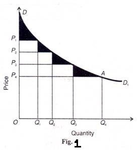
(2) To deal with each buyer on a take-it-or-leave-it basis. When the discriminator of first degree is able to deal with his customers on the above basis, he can transfer the whole of consumers’ surplus to himself. Consider Figure 1. Where DD1 is the demand curve faced by the monopolist. Each buyer is assumed as a price-taker. Suppose the discriminating monopolist sells four units of his product at four different prices:

OQ1 unit at OP1price, Q1Q2 unit at OPprice, Q2Q3 unit at OP3 price and Q3Q4 unit at OP4 price. The total revenue (or price) obtained by him would be OQ4 AD. This area is the maximum expenditure that the consumers are willing to incur to buy all four units of the product under the first-degree discriminator’s all-or-nothing offer. But with no price discrimination under simple monopoly, the monopolist would sell all four units at the uniform price OP4 and thus obtain the total revenue of OQ4AP4.

This area represents the total expenditure that consumers would actually pay for the four units. Thus the difference between what Quantity the consumers were willing to pay (OQ4 AD) under Fig. 1 the take-it-or-leave-it offer of the first degree discrimi­nator and what they actually pay (OQ4AP4) to the simple monopolist, is consumers’ surplus. This is equal to the area of the triangle DAP4.

Thus under the first-degree price discrimination, the entire consumers’ surplus is pocketed by the monopolist when he charges a separate price for each unit of the product. Price discrimination of the first degree is rare and is to be found in such rare products as diamonds, jewels, precious stones, etc. But a monopolist must have full knowledge of the demand curve faced by him and he should know the maximum price that the consumers are willing to pay for each unit of the product he wants to sell.

Discrimination of the Second Degree (2nd) or Multi-part Pricing

In discrimination of the second degree, the monopolist divides the consumers in different slabs or groups or blocks and charges different prices for different slabs of the same product. Since the earlier units of the product have more utility for the consumers than the later ones, the monopolist charges a higher price for the former units and reduces the price for the later units in the respective slabs.

Such discrimination is only possible if the demand of each consumer below a certain maximum price is perfectly inelastic. Electric supply companies in developed countries practice discrimination of the second degree when they charge a high rate for the first slab of kilowatts of electricity consumed. As more electricity is used, the rate falls with subsequent slabs.

Figure 2 illustrates the second degree discrimination, where DD1is the demand curve for electric­ity on the part of domestic consumers in a town. CP3 represents the cost of generating electricity, so that the electricity company charges M1P1 rate per kw. up to OM1 units. For consuming the next M1 to М2 units, the rate is lowered to M2P2. The lowest rate charged is M3P3 for M2 to M3 units. M3P3 is, however, the lowest rate which will be charged even if a con­sumer consumes more than M3 units of electricity.

If the electricity company were to charge only one rate throughout, say M3P3the total revenue would not be maximized. It would be OCP3 M3But by charg­ing different rates for different unit slabs, it gets the total revenue equal to OM3 x P1M1 + OM2 x P2M2 + OM3x P3M3 Thus the second degree discriminator would take away a part of consumers’ surplus covered by the rectangles ABEP1and BCFP2 .The shaded area in three triangles DAP1 Р1ЕР2, and P2FP3 still remains with consumers as their surplus.

The second degree price discrimination is practised by telephone companies, railways, companies supplying water, electricity and gas in developed countries where these services are available in plenty. But it is not found in developing countries like India where such services are scarce.

The differences between the first and second degree price discrimination may be noted. In the first degree discrimination, the monopolist charges a different price for each different unit of the prod­uct. But in second degree discrimination, a number of units in one slab (or group or block) are sold at the lowest price and as the slabs increase, the prices charged by the monopolist are lowered. In the case of the former the monopolist takes away the whole of consumers’ surplus. But in the latter case, the monopolist takes away only a portion of the consumers’ surplus and the other portion is left with the buyer.

Conditions under which Price Discrimination is Possible

Price discrimination is possible under following conditions:

  1. Nature of Commodity

In the first place it is said that price discrimination is possible when the nature of the commodity or service is such that there is no possibility of transference from one market to the other.

That is, the goods sold in the cheaper market cannot be resold in the dearer market; otherwise the monopolist’s purpose will be defeated.

  1. Distance of Two Markets

Price discrimination is possible when the two markets or markets are separated by large distance or tariff barriers, so that it is not possible to transfer goods from a cheaper market to dearer markets. For instance, a monopolist may sell the same product at a higher price in Bombay and lower price in Meerut.

  1. Ignorance of the Consumers

Price discrimination is possible when the consumers are ignorant about price discrimination, they are not aware that in one part of the market prices are lower than in the other part. Thus, he purchases in dearer market, than in cheaper market since he is ignorant of the prices that are prevailing in different markets.

  1. Government Regulation

Price discrimination occurs when the government rules and regulations permit. For instance, according to rules, electricity rates are fixed at higher level for industrial purposes and lower for domestic uses. Similarly, railways charge by law higher fares from first class passengers than from the second class passengers. Hence, price discrimination is possible because of legal sanction.

  1. Geographical Discrimination

Price discrimination may be possible on account of geographical situations. The monopolist may discriminate between home and foreign buyers by selling at lower price in the foreign market than in the domestic market. Geographical discrimination is possible because no unit of the commodity sold in one market can be transferred to another.

  1. Difference in Elasticity of Demand

A commodity may have different elasticity of demand in different markets. Thus, the market of a commodity can be separated on the basis of its elasticity of demand.

Hence, a monopolist can charge different prices in different markets classified on the basis of elasticity of demand, low price is charged where demand is more elastic and high price in the market with the less elastic demand or inelastic demand.

  1. Artificial Difference between Goods

A monopolist may create artificial differences by presenting the same commodity under different names and labels, one for the rich and snobbish buyers and the other for the ordinary customers. For instance, a biscuit manufacturer may wrap small quantity of the biscuits, give it separate name and charge a higher price. Thus, he may charge different price for substantially the same product. He may charge Rs. 2/- for 100 gram wrapped biscuits and Rs. 1.50 for unwrapped biscuits.

Production: Meaning, Factors of Production, Production Function, Features, Types

Production is the process of creating goods and services by utilizing various resources. It involves combining inputs such as labor, capital, raw materials, and entrepreneurship to produce output that satisfies human wants and needs. The goal of production is to maximize efficiency, minimize costs, and generate value, contributing to economic growth and development. It is a key concept in economics as it drives the creation of wealth and the distribution of goods in a society.

Factors of Production:

  • Land:

Refers to all natural resources used in the production process, including raw materials like water, minerals, forests, and agricultural land. It is the base for extracting resources that are essential for creating goods and services.

  • Labour:

The human effort, both physical and mental, applied in the production process. Labor includes workers at all skill levels, from manual laborers to highly skilled professionals, and their efforts are rewarded in the form of wages or salaries.

  • Capital:

The tools, machinery, buildings, and technology used in the production of goods and services. Capital enhances the efficiency of labor and helps increase productivity, which in turn contributes to economic growth.

  • Entrepreneurship:

The ability to organize the other factors of production and take on the risks associated with starting and running a business. Entrepreneurs innovate, create new products, and take the initiative to bring together resources for production.

  • Knowledge:

Refers to technical know-how, expertise, and skills that influence the efficiency of production. This includes education, training, and research that enhance the ability to optimize the use of other factors of production.

  • Technology:

The tools, systems, and methods used to improve production efficiency and the quality of output. Technological advancements often lead to cost reductions, higher productivity, and the creation of new products or services.

Production Function

Production Function is an economic concept that describes the relationship between the inputs used in production and the resulting output. It shows how different combinations of labor, capital, and other factors of production contribute to the production of goods or services. The production function helps in understanding the efficiency of resource utilization, and how changes in the quantity of inputs affect the level of output. It is often expressed as an equation or graph, representing the technological relationship in production.

Mathematically, such a basic relationship between inputs and outputs may be expressed as:

Q = f( L, C, N )

Where

Q = Quantity of output

L = Labour

C = Capital

N = Land.

Hence, the level of output (Q), depends on the quantities of different inputs (L, C, N) available to the firm. In the simplest case, where there are only two inputs, labour (L) and capital (C) and one output (Q), the production function becomes.

Q = f(L, C)

“The production function is a technical or engineering relation between input and output. As long as the natural laws of technology remain unchanged, the production function remains unchanged.” Prof. L.R. Klein

“Production function is the relationship between inputs of productive services per unit of time and outputs of product per unit of time.” Prof. George J. Stigler

“The relationship between inputs and outputs is summarized in what is called the production function. This is a technological relation showing for a given state of technological knowledge how much can be produced with given amounts of inputs.” Prof. Richard J. Lipsey

Thus, from the above definitions, we can conclude that production function shows for a given state of technological knowledge, the relation between physical quantities of inputs and outputs achieved per period of time.

Features of Production Function

Following are the main features of production function:

  1. Substitutability

The factors of production or inputs are substitutes of one another which make it possible to vary the total output by changing the quantity of one or a few inputs, while the quantities of all other inputs are held constant. It is the substitutability of the factors of production that gives rise to the laws of variable proportions.

  1. Complementarity

The factors of production are also complementary to one another, that is, the two or more inputs are to be used together as nothing will be produced if the quantity of either of the inputs used in the production process is zero.

The principles of returns to scale is another manifestation of complementarity of inputs as it reveals that the quantity of all inputs are to be increased simultaneously in order to attain a higher scale of total output.

  1. Specificity

It reveals that the inputs are specific to the production of a particular product. Machines and equipment’s, specialized workers and raw materials are a few examples of the specificity of factors of production. The specificity may not be complete as factors may be used for production of other commodities too. This reveals that in the production process none of the factors can be ignored and in some cases ignorance to even slightest extent is not possible if the factors are perfectly specific.

Production involves time; hence, the way the inputs are combined is determined to a large extent by the time period under consideration. The greater the time period, the greater the freedom the producer has to vary the quantities of various inputs used in the production process.

In the production function, variation in total output by varying the quantities of all inputs is possible only in the long run whereas the variation in total output by varying the quantity of single input may be possible even in the short run.

Time Period and Production Functions

The production function is differently defined in the short run and in the long run. This distinction is extremely relevant in microeconomics. The distinction is based on the nature of factor inputs.

Those inputs that vary directly with the output are called variable factors. These are the factors that can be changed. Variable factors exist in both, the short run and the long run. Examples of variable factors include daily-wage labour, raw materials, etc.

On the other hand, those factors that cannot be varied or changed as the output changes are called fixed factors. These factors are normally characteristic of the short run or short period of time only. Fixed factors do not exist in the long run.

Consequently, we can define two production functions: short-run and long-run. The short-run production function defines the relationship between one variable factor (keeping all other factors fixed) and the output. The law of returns to a factor explains such a production function.

For example, consider that a firm has 20 units of labour and 6 acres of land and it initially uses one unit of labour only (variable factor) on its land (fixed factor). So, the land-labour ratio is 6:1. Now, if the firm chooses to employ 2 units of labour, then the land-labour ratio becomes 3:1 (6:2).

The long-run production function is different in concept from the short run production function. Here, all factors are varied in the same proportion. The law that is used to explain this is called the law of returns to scale. It measures by how much proportion the output changes when inputs are changed proportionately.

Types of Production Function:

1. Short-Run Production Function

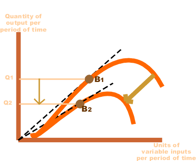
In the short run, at least one input is fixed (usually capital), while other inputs (like labor) are variable. The short-run production function examines how changes in variable inputs affect output, keeping the fixed input constant.

Key Features:

  • Focuses on the law of variable proportions (diminishing marginal returns).
  • Output increases initially at an increasing rate, then at a decreasing rate, and eventually may decline.

Example:

A factory with fixed machinery (capital) adds more workers (labor). Initially, productivity increases, but as workers crowd the factory, additional output diminishes.

2. Long-Run Production Function

In the long run, all inputs are variable, allowing firms to adjust labor, capital, and other resources fully. The long-run production function focuses on the optimal combination of inputs to achieve maximum efficiency and output.

Key Features:

  • Examines returns to scale:
    • Increasing Returns to Scale: Doubling inputs results in more than double the output.
    • Constant Returns to Scale: Doubling inputs results in a proportional doubling of output.
    • Decreasing Returns to Scale: Doubling inputs results in less than double the output.
  • Useful for long-term planning and investment decisions.

3. Cobb-Douglas Production Function

A mathematical representation of the relationship between two or more inputs (e.g., labor and capital) and output. It is commonly expressed as:

Q = A*L^α*K^β*

Where:

  • Q: Total output
  • L: Labor input
  • K: Capital input
  • α,β: Elasticities of output with respect to labor and capital
  • A: Total factor productivity

Key Features:

  • Demonstrates the contribution of labor and capital to output.
  • Widely used in economics for empirical studies and forecasting.

4. Fixed Proportions Production Function (Leontief Production Function)

In this type, inputs are used in fixed proportions to produce output. Increasing one input without proportionately increasing the other does not lead to higher output.

Example:

A car requires one engine and four tires. Adding more engines without increasing the number of tires will not produce more cars.

5. Variable Proportions Production Function

Inputs can be substituted for one another in varying proportions while producing the same level of output.

Example:

A firm can use either more machines and less labor or more labor and fewer machines to produce the same output.

6. Isoquant Production Function

An isoquant represents all possible combinations of two inputs (e.g., labor and capital) that produce the same level of output. The isoquant approach analyzes how inputs can be substituted while maintaining output levels.

Key Features:

  • Focuses on input substitution.
  • Helps determine the least-cost combination of inputs for a given output.

Elasticity of Demand: Meaning, Types and Significance

Elasticity of Demand refers to the responsiveness of the quantity demanded of a good or service to changes in its price. It measures how much the demand for a product changes when there is a change in its price. If demand changes significantly with a small price change, the demand is considered elastic. If the demand changes little or not at all, it is inelastic. The elasticity of demand is calculated as the percentage change in quantity demanded divided by the percentage change in price. This concept helps businesses and economists understand consumer behavior and pricing strategies.

Types of Elasticity:

Distinction may be made between Price Elasticity, Income Elasticity and Cross Elasticity. Price Elasticity is the responsiveness of demand to change in price; income elasticity means a change in demand in response to a change in the consumer’s income; and cross elasticity means a change in the demand for a commodity owing to change in the price of another commodity.

(a) Infinite or Perfect Elasticity of Demand

Let as first take one extreme case of elasticity of demand, viz., when it is infinite or perfect. Elasticity of demand is infinity when even a negligible fall in the price of the commodity leads to an infinite extension in the demand for it. In Fig. 1 the horizontal straight line DD’ shows infinite elasticity of demand. Even when the price remains the same, the demand goes on changing.

(b) Perfectly Inelastic Demand

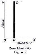
The other extreme limit is when demand is perfectly inelastic. It means that howsoever great the rise or fall in the price of the commodity in question, its demand remains absolutely unchanged. In Fig. 2, the vertical line DD’ shows a perfectly inelastic demand. In other words, in this case elasticity of demand is zero. No amount of change in price induces a change in demand.

In the real world, there is no commodity the demand for which may be absolutely inelastic, i.e., changes in its price will fail to bring about any change at all in the demand for it. Some extension/contraction is bound to occur that is why economists say that elasticity of demand is a matter of degree only. In the same manner, there are few commodities in whose case the demand is perfectly elastic. Thus, in real life, the elasticity of demand of most goods and services lies between the two limits given above, viz., infinity and zero. Some have highly elastic demand while others have less elastic demand.

(c) Very Elastic Demand

Demand is said to be very elastic when even a small change in the price of a commodity leads to a considerable extension/con­traction of the amount demanded of it. In Fig. 3, DD’ curve illustrates such a demand. As a result of change of T in the price, the quantity demanded extends/contracts by MM’, which clearly is comparatively a large change in demand.

(d) Less Elastic Demand

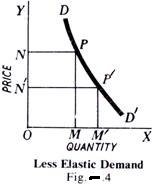
When even a substantial change in price brings only a small extension/contraction in demand, it is said to be less elastic. In Fig. 4, DD’ shows less elastic demand. A fall of NN’ in price extends demand by MM’ only, which is very small.

Significance of Elasticity of Demand

  1. Determination of Output Level

For making production profitable, it is essential that the quantity of goods and services should be produced corresponding to the demand for that product. Since the changes in demand are due to the change in price, the knowledge of elasticity of demand is necessary for determining the output level.

  1. Determination of Price

The elasticity of demand for a product is the basis of its price determination. The ratio in which the demand for a product will fall with the rise in its price and vice versa can be known with the knowledge of elasticity of demand.

If the demand for a product is inelastic, the producer can charge high price for it, whereas for an elastic demand product he will charge low price. Thus, the knowledge of elasticity of demand is essential for management in order to earn maximum profit.

  1. Price Discrimination by Monopolist

Under monopoly discrimination the problem of pricing the same commodity in two different markets also depends on the elasticity of demand in each market. In the market with elastic demand for his commodity, the discriminating monopolist fixes a low price and in the market with less elastic demand, he charges a high price.

  1. Price Determination of Factors of Production

The concept of elasticity for demand is of great importance for determining prices of various factors of production. Factors of production are paid according to their elasticity of demand. In other words, if the demand of a factor is inelastic, its price will be high and if it is elastic, its price will be low.

  1. Demand Forecasting

The elasticity of demand is the basis of demand forecasting. The knowledge of income elasticity is essential for demand forecasting of producible goods in future. Long- term production planning and management depend more on the income elasticity because management can know the effect of changing income levels on the demand for his product.

  1. Dumping

A firm enters foreign markets for dumping his product on the basis of elasticity of demand to face foreign competition.

  1. Determination of Prices of Joint Products

The concept of the elasticity of demand is of much use in the pricing of joint products, like wool and mutton, wheat and straw, cotton and cotton seeds, etc. In such cases, separate cost of production of each product is not known.

Therefore, the price of each is fixed on the basis of its elasticity of demand. That is why products like wool, wheat and cotton having an inelastic demand are priced very high as compared to their byproducts like mutton, straw and cotton seeds which have an elastic demand.

  1. Determination of Government Policies

The knowledge of elasticity of demand is also helpful for the government in determining its policies. Before imposing statutory price control on a product, the government must consider the elasticity of demand for that product.

The government decision to declare public utilities those industries whose products have inelastic demand and are in danger of being controlled by monopolist interests depends upon the elasticity of demand for their products.

  1. Helpful in Adopting the Policy of Protection

The government considers the elasticity of demand of the products of those industries which apply for the grant of a subsidy or protection. Subsidy or protection is given to only those industries whose products have an elastic demand. As a consequence, they are unable to face foreign competition unless their prices are lowered through sub­sidy or by raising the prices of imported goods by imposing heavy duties on them.

  1. Determination of Gains from International Trade

The gains from international trade depend, among others, on the elasticity of demand. A country will gain from international trade if it exports goods with less elasticity of demand and import those goods for which its demand is elastic.

In the first case, it will be in a position to charge a high price for its products and in the latter case it will be paying less for the goods obtained from the other country. Thus, it gains both ways and shall be able to increase the volume of its exports and imports.

Lucknow University BBA Notes

>>New NEP 2024-25 Syllabus Notes<<

1st Semester
P1 Principles of Management (Updated) VIEW
P2 Business Statistics (Updated) VIEW
P3 Financial Accounting (Updated) VIEW
P4 Business Communication (Updated) VIEW
P5 Computer and IT Applications-I (Updated) VIEW
CC1 Personality Development and Grooming (Updated) VIEW
2nd Semester
P6 Organizational Behaviour (Updated) VIEW
P7 Managerial Economics (Updated) VIEW
P8 Cost and Management Accounting (Updated) VIEW
P9 Business Environment (Updated) VIEW
P10 Indian Constitution (Updated) VIEW
VC1 Resume Writing and Corporate Communication (Updated) VIEW
3rd Semester
P11 Financial Management (Updated) VIEW
P12 Operations Management (Updated) VIEW
P13 Marketing Management (Updated) VIEW
P14 Human Resource Management (Updated) VIEW
P15 Computer and IT Applications-II (Updated) VIEW
CC2 Interview Preparation and Planning (Updated) VIEW

4th Semester

P16 E-Commerce (Updated) VIEW
P17 Logistic and Supply Chain Management (Updated) VIEW
P18 Customer Relationship Management (Updated) VIEW
P19 Industrial Relations Management (Updated) VIEW
VC2 Role Play and Simulation (Updated) VIEW

>>NEP 2021-22 Syllabus Notes<<

1st Semester

Principles of Management (Updated) VIEW
Financial & Management Accounting-I (Updated) VIEW
Business Organisations (Updated) VIEW
Business Communication (Updated) VIEW
Computer & IT Applications-I (Updated) VIEW
Personality Development and Grooming (Updated) VIEW

2nd Semester

Organizational Behaviour (Updated) VIEW
Financial & Management Accounting-II (Updated) VIEW
Managerial Economics (Updated) VIEW
Business Environment (Updated) VIEW
Quantitative Techniques-I (Updated) VIEW
Resume Writing and Corporate Communication (Updated) VIEW

3rd Semester

Financial Management (Updated) VIEW
Marketing Management (Updated) VIEW
Operations Management (Updated) VIEW
Human Resource Management (Updated) VIEW
Computer & IT Applications-II (Updated) VIEW
Interview Preparation & Planning (Updated) VIEW

4th Semester

Taxation & Laws (Updated) VIEW
Customer Relationship Management (Updated) VIEW
Logistic and Supply Chain Management (Updated) VIEW
Industrial Relations Management (Updated) VIEW
Quantitative Techniques-II (Updated) VIEW
Role Play and Simulation (Updated) VIEW

5th Semester

Entrepreneurship and Family Business-I (Updated) VIEW
Business Ethics (Updated) VIEW
Business Policy & Strategic Management-I (Updated) VIEW
Business Laws (Updated) VIEW
Financial Institutions (Updated) VIEW
Consumer Behaviour (Updated) VIEW

6th Semester

Entrepreneurship and Family Business-II (Updated) VIEW
Corporate Governance and Corporate Social Responsibility (Updated) VIEW
Business Policy & Strategic Management-II (Updated) VIEW
Management Information System (Updated) VIEW
E-Commerce (Updated) VIEW
Talent Management and HRIS (Updated) VIEW

7th Semester

Decision Sciences (Updated) VIEW
Project Management (Updated) VIEW
Business Analytics (Updated) VIEW
Banking Operations Management (Updated) VIEW
Retail & Rural Marketing (Updated) VIEW
Insurance & Risk Management (Updated) VIEW
Service and Industrial Marketing (Updated) VIEW
Research Methodology (Updated) VIEW

>Old Syllabus<

1st Semester

Subjects

BBA101 Business Mathematics (No Update)

VIEW

BBA102 Computer Fundamentals (Updated)

VIEW

BBA103 Financial Accounting (Updated)

VIEW

BBA104 Managerial Economics (Updated)

VIEW

BBA105 Marketing Fundamentals (Updated)

VIEW

BBA106 Principles of Management (Updated)

VIEW

2nd Semester

Subjects

BBA201 Business Communication (Updated)

VIEW

BBA202 Business Statistics (Updated)

VIEW

BBA203 Foreign Trade of India (Updated)

VIEW

BBA204 Environmental Studies (Updated)

VIEW

BBA205 Financial Mathematics (Updated)

VIEW

BBA206 Indian Value System (Updated)

VIEW

3rd Semester

Subjects

BBA301 Advertising Management (Updated)

VIEW

BBA302 Banking operations Management (Updated)

VIEW

BBA303 Business Environment (Updated)

VIEW

BBA304 Management Accounting (Updated)

VIEW

BBA305 Organizational Behavior (Updated)

VIEW

BBA306 Research Methodology (Updated)

VIEW

4th Semester

Subjects

BBA401 Business Laws (Updated)

VIEW

BBA402 Financial Management (Updated)

VIEW

BBA403 Human Resource Management (Updated)

VIEW

BBA404 Information Management (Updated)

VIEW

BBA405 Operation Management (Updated)

VIEW

BBA406 Consumer Behavior (Updated)

VIEW

5th Semester

Subjects

BBA501 E-Commerce (Updated)

VIEW

BBA502 Financial Services (Updated)

VIEW

BBA503 Insurance and Risk Management (Updated)

VIEW

BBA504 Retail & Rural Marketing (Updated)

VIEW

BBA505 Taxation Laws (Updated)

VIEW

BBA506 Managing Personal Finance (Updated)

VIEW

6th Semester

Subjects

BBA601 Business Policy (Updated)

VIEW

BBA602 Company Law (Updated)

VIEW

BBA603 Entrepreneurship (Updated)

VIEW

BBA604 International Business (Updated)

VIEW

BBA605 Marketing of Service (Updated)

VIEW

BBA606 Project Management (Updated)

VIEW

error: Content is protected !!