Year: 2020

Sales promotion refers to ‘those marketing activities that stimulate consumer shows and expositions.

Purchasing and dealer effectiveness such as displays, demonstration and various non- recurrent selling efforts not in the ordinary routine.” According to A.H.R. Delens: “Sales promotion means any steps that are taken for the purpose of obtaining an increasing sale. Often this term refers specially to selling efforts that are designed to supplement personal selling and advertising and by co-ordination helps them to become more effective.”

In the words of Roger A. Strong, “Sales promotion includes all forms of sponsored communication apart from activities associated with personal selling. It, thus includes trade shows and exhibits, combining, sampling, premiums, trade, allowances, sales and dealer incentives, set of packs, consumer education and demonstration activities, rebates, bonus, packs, point of purchase material and direct mail.”

Objectives of Sales Promotion:

Sales promotion is a vital bridge or a connecting link between personal selling and advertising.

Sales promotion activities are undertaken to achieve the following objectives:

1. To increase sales by publicity through the media which are complementary to press and poster advertising.
2. To disseminate information through salesmen, dealers etc., so as to ensure the product getting into satisfactory use by the ultimate consumers.
3. To stimulate customers to make purchases at the point of purchase.
4. To prompt existing customers to buy more.
5. To introduce new products.
6. To attract new customers.
7. To meet competition from others effectively.
8. To check seasonal decline in the volume of sales.

Importance of Sales Promotion:

The importance of sales promotion has increased tremendously in the modern times. Lakhs of rupees are being spent on sales promotional activities to attract the consumers in our country and also in other countries of the world.

Some large companies have also begun to appoint sales promotion managers to handle miscellaneous promotional tools. All these facts show that the importance of sales promotion activities is increasing at a faster rate.

As in the case of advertising, effective sales promotion involves an on-going process with a number of stages.

1. Establishment of objectives:

Sales-promotion objectives vary according to the target market. If the target is the customer, objectives could include the encouragement of increased usage or the building of trial among non-users or other brand users. For intermediaries, objectives could be to encourage off-season sales or offsetting competitive promotions. Sales-promotion activity could also be aimed at internal personnel, making up part of the reward system

2. Selection of promotional tools:

Promotional objectives form the basis for selecting the most appropriate sales-promotion tools. The cost and effectiveness of each tool must be assessed with regard to achieving these objectives in respect of each target market. The tools available to the service marketer are described in more detail in the next section.

3. Planning the sales-promotion programme:

The major decisions that need to be made when designing the sales-promotion programme relate to the timing of the promotion and how long this tool is to be used. Also important are the size of incentive, rules for eligibility and, of course, the overall budget for the promotion.

4. Pre-testing:

This needs to be undertaken to ensure that potentially expensive problems are discovered before the full launch of a promotion. Testing in selected market segments can highlight problems of ambiguity, response rates and give an indication of cost effectiveness.

5. Implementation:

The programme for implementation must include two important time factors First, it must indicate the ‘lead time’- the time necessary to bring the programme up to the point where the incentive is made available to the public. Second, the ‘sell in time’ which is the period of time from the date of release to when approximately 90-95 per cent, of incentive material has been received by potential customers.

6. Evaluation:

The performance of the promotion needs to be assessed against the objectives set. If objectives are specific and quantifiable, measurement would seem to be easy. However, extraneous factors could account for the apparent success of many sales-promotion activities.

For example, competitive actions or seasonal variations may have influenced customers’ decision making. It can also be extremely difficult to separate out the effects of sales-promotion activity from other promotional activity-or indeed from other marketing-mix changes.

Steps in Personal Selling

The selling process consists of several steps; there are few basic steps, which need to be followed for all types of products. The selling process can be for short time or long time, depending upon the nature of the product. A product, which needs huge investment, may take longer time to complete the selling process whereas in case of daily products where the customer is aware of the nature of the product, the selling process ends in shorter time.

Example: Door to door sales, where the salesperson explains all the steps and ends the process in 10 to 15 minutes. However, for heavy machinery, it may take time to present the technical nature and explain the product; it takes more than one visit to complete the selling process.

Prospecting

The initial step of selling process starts with prospecting or searching for potential customers. Apart from retail sales, it’s very rare when customers reach out to the salesperson. It’s the salesperson who reaches out to customers in order to sell the product.

The following are the two major activities under prospecting:

• Find the prospects or the potential customers
• Educate them in order to figure out if they are valid customers

Find the Prospects or the Potential Customers

Finding the prospect is not an easy step for a sales person because consumers would not even like to listen to the presentation regarding the product they do not need. The rate of saying “No” is very high. In few consumer goods, the identification of customers comes from sources like friends, relatives, colleagues etc. The following are some of the best sources.

• Existing Customers” One of the good sources of prospects is an existing customer. For a salesperson, it is very easy to sell the products to an existing customer instead of selling to the new customers.
• Never-ending Chain” This is a competing strategy to find out prospects. The salesperson reaches many new customers with the help of existing customers. The salesperson selling the product to existing customers asks to provide referral to friends or relatives and the salesperson reaches the new customers. This chain goes on and on.
• Cold Call: In this technique, the salesperson has to visit door to door to sell the products. The sales process starts from introduction but in this case, the rejection rate is high.
• Directories: The salesperson tries to find out prospect customer contact with the help of a directory. The salesperson can also collect the information through membership directories of trade associations, social organization etc.
• Mailing: The companies promote their product through mails by sending advertisements. The advantage is that it’s cheap and the company targets many customers by sending mass mailers.
• Exhibition: The salesperson could target the prospective customers through tradeshows and exhibitions. It’s one of the simplest ways and the salesperson could also practically show the use of the product and the features. Announcement is advance, before the exhibitions starts, is very helpful to attract more customers.

Train/Educate the Prospects

After the salesperson has identified the potential customers, he should find out if they are valid prospects. After finding the valid prospects, the salesperson has to give the presentation.

There are several approaches for qualifying customers and the prominent approach is MAN, i.e., Money, Authority and Need.

• Money: The salesperson should know the financial status of the customers because money matters a lot, and, without it, the prospect cannot purchase the product. The consumer or the prospect should be able to pay money in return of the product.
• Authority: The prospect that is purchasing the product should have the authority to make decision. This is important while dealing with government agencies, corporate etc.
• Need: This is one of the most important points because if the prospect has money and also the authority but there is no need of the product, he or she will not purchase the product.

The salesperson has to find out about these aspects before proceeding to the selling process.

Preparation for the Sale of Product

Once the prospect has been identified and qualified as discussed in first step, the salesperson has to prepare for the sales of product or service. The following are the two stages involved in preparation −

• Pre-approach
• Call Planning

Pre-approach

This step involves collecting all the information important to learn about the prospects and their needs. The following are the four steps of pre-approach:

• Prospect need and ability should be disclosed.
• All the required information, which would help the salesperson to prepare the presentation.
• Relevant information, which helps salesperson not create any errors during presentation.
• Confidence to tackle the questions of the prospect.

Call Planning

Call Planning includes a particular planning sequence. The salesperson calls the customer and explains the objective of the call and explains the product to makes appointments.

The first objective of the salesperson is to get an order from the customer. Some objectives may also be required in the mid-of-the-call progress, depending on the call. Following are a few objectives for call planning −

• Collect more information from the customer .
• Find out the need of the customer and link with the features of product.
• Take permission from customer before presentation of product.
• Suggest a new distributor.

The salesperson has to develop a strategy and plan accordingly to achieve the objective or goal. The salesperson should be very careful while checking the background of the customers and obtaining details. This helps to frame a strategy and develop a plan. The calls made by salesperson are costly, so they have to take prior appointment.

Presentation

In this step, the salesperson has to give the presentation regarding the product to the customer. She/he should explain the features of the product and how it will fulfill the needs. The presentation should be clear and understandable by the customer. It should also be interesting to keep the customer involved in the conversation.

A presentation can be classified into the following categories −

• Fully automated
• Semi-automated
• Memorized
• Organized
• Unstructured

Fully Automated

In this approach, the salesperson gives the presentation with the help of slides in a structured manner. He also explains and clears the doubts of the customers. Example: Life Insurance.

Semi-Automated

The salesperson reads out the company brochures and adds comments as per requirement or queries from the client. Example: Pharmaceutical products.

Memorized

The company presents its message, which is short and crisp, and which can be easily memorized by the customer.

Organized

One of the most attractive, effective and often-used approaches is organized presentation. The salesperson can make changes in the presentation as required but based on the company’s pre-defined outline. In this approach, the sale person covers the four steps, i.e., Attention, Interest, Desire and Action.

Unstructured

The salesperson and the customer together try to resolve the problems. Hence this approach is also known as problem solving. This type of presentation is not well focused many a times; some points are missed and time is wasted. Also the salesperson has to face many queries from the customers and if the salesperson is new in the field, he/she will not be able to answer the queries in an effective manner.

Thus, we can conclude that the presentation to the established customers should be done by an effective salesperson.

Handling Objections

The salesperson has to struggle to sell the product to the customers. During the sales process, the prospects raise objections, which can be stated or hidden. Prospects may state the reason for objections and give a chance to salesperson to answer. This is an absolute situation because the prospect is informed regarding the objections.

Unfortunately, in many cases, the prospects do not provide the reason for objection of the product. They hide their real reason for not buying the product. If the salesperson is unable to know the real reason, he/she will not be able to resolve the problem.

To resolve this, there are two techniques to find out the objections.

• To allow the prospect to talk to find out the hidden objection.
• The observation gained by experience and mixing with the knowledge of the prospects.

Many times, the objection is due to high price of the product. That objection can be answered when the salesperson has the knowledge of the competitor’s products as well.

Also, in many cases, the prospects do not understand the technical aspects and are misinformed. The salesperson should provide additional information in this case.

Now we can conclude that the objection can be resolved by providing an alternative product to the prospects.

Closing the Sale

After answering the objections made by prospects, the salesperson asks for the prospect to order the product. If the prospect does not agree to buy the product, the entire effort gets waste. The following are some effective techniques to close the sale:

Gift Close

In this technique, the customers get an incentive for immediate buying action. The salesperson informs regarding the benefits of the product to the prospects.

Example: A company provides an option to the prospect that if the bill exceeds Rs.3000, he can buy a bed sheet worth 2000 for just Rs.200.

Here, if the customer has made a purchase of Rs.2500, he will check out to buy something else to reach 3000. This helps the company to sell two extra products — one for Rs.500 or more to reach 3000 and another, bed sheet for Rs.200.

Direct Close

This is one of the simplest techniques to close the sales. This happens when the buyer has positive approach to buy a product. The salesperson summarizes the important points that were made prior to sale.

Example: A prospect needs beauty cream and steps into a shop. The salesperson offers the products; if required, shows the demo. Once the prospect is satisfied, he/she will buy it.

If the salesperson is experienced, he/she will try to close it as early as possible because he/she would understand if the prospect is inclined to buy the product. A good salesperson makes sure that he has completed all the steps during sales process.

Thus, closing is an important step in sales process. The other steps are meaningless without closing.

Follow-up

After making the sale, the salesperson has to follow up with the prospects. After sales activities are important parts of the selling process. This helps in reducing any doubt by the customer regarding the product or service. There is also a chance that the buyer with buy again in future.

There are specific policies by a company for after sales activities. Even though the company provides good products, there will be few complaints from customers. The complaints should be taken seriously and the company should try to resolve. This helps the company to improve in terms of product or service.

An experienced salesperson tries to provide the best service to its customers. As a part of handling complaints, they also keep the prospect informed regarding the latest products or services and also provide other types of assistance. The salesperson should build good rapport with the customer. This helps to get more customers because the existing customer will refer to his friends and relatives.

The salesperson should thank the customer for the business and offer small gifts.

1. Self confidence and polite

Self-confidence is the first step to success. Be confident; if you are not sure yourselves, how can you convince your customer. Self confidence is not arrogance, be polite.

2. Commitment

You have to commit to your job, this industry is too tough for those who has only half-hearted, committed or choose another field, do not waste your time.

3. Discipline

Do not expect a “hit and run” system can bring any result, you should have discipline to follow up all your commitment.

4. Honest and Enthusiastic

All you tell should be the truth, but does not mean you have to tell all the truth which you have to keep due to positioning and negotiation. Do not over promise, if you are not sure, tell them I will find the answer for you.

5. Give impact

There are two many sales knocking at your customers’ door, they can only remember the sales executive who give them an impact (either good or bad).

6. Preparation

A good impact can only achieved if you prepare properly. I will not see any High Way salesman who just drop in and  hear him talking nonsense, but I will accept somebody who has prepared a relevant topic which can arouse my interest (to get more value from him/her). No preparation do not go to see the customer, you waste you time and the company money.

7. Keep on learning

Every day we learn, we can only advise our customers if we know what they are current doing. And usually you learn more from your customers (on field learning) by asking relevant question, but before you can ask relevant questions you should have some basic knowledge on the issue.

8. Convey your idea to your customer

You should have a courage to convey your idea, not just “Yes, Sir”, you will lose your value if every time your response is “Yes, Sir”, then the customer will send you away with1 kg of spray powder or ink. Usually, most of the idea comes from your observation/listen from others customer. By systematically learning, you can obtain a lot of idea.

9. Be creative and pro active

Don’t bring the same topic every time you visit your customer, otherwise you become Order Taker and they will happily send you away with 1 kg of spray powder. Think of different topic, (ink, graphic supplier, logistic, business environment, competition, payment, pricing, investment, interest rate, capital etc.). The more knowledge you know on your relevant field, the more your customer will value you.

• Killer instinct alias closing sales

Whatever value you add to the customer, some body has to pay and it is your customer who is going to pay. If you can’t close the sales, you have to question yourself: does my customer aware of my value?

Qualities of Highly affective Sales executive

1. Ability to define the position’s exact functions and duties in relation to the goals the company should expect to attain. Sales executives calculate what is entailed in their responsibilities. Whether or not the company provides them with a job description, they draw up their own descriptions consistent with the responsibilities assigned by higher management. Revision are necessary whenever changes occur in the assigned responsibilities or in company goals.
2. Ability to utilize time efficiently. The time of sales executives is valuable, and they budget it and use it carefully. They allocate working time to tasks yielding the greatest return. They arrive at an optimum division between office work and field supervision. Even the use of off duty hours is important. Excessive work time and too little leisure reduces efficiency. Successful sales executive balance such leisure time activities as community service and professional meeting against personal social activates, recreation, and self improvement.
3. Ability to select and train capable subordinates and willingness to delegate sufficient authority to enable them to carry out assigned task with minimum supervision. Ability to delegate authority is must. Effective executives select high caliber subordinates and provide them with authority to make decisions. Within existing policy limits, decision are made by subordinates; when an exception falling outside these limits occurs, the superior decides. The more capable the subordinates, the wider policy limits can be And the more the superior’s time is freed for planning.
4. Ability to exercise skilled leadership. Competent sales executives develop and improve their skills in dealing with people although they rely to a certain extent on an intuitive grasp of leadership skills, they depend far move on careful study of motivational factors and shrewd analysis of the ever changing patterns of unsatisfied needs among those with whom they work. Skilled leadership is important in dealing with subordinates and with everyone else.
5. Ability to allocate sufficient time for thinking and planning. Able administrators make their contributions through thinking and planning. They know how and are willing to think. They recognize that reviewing past performances is a prerequisite to planning. They strive to gain new insight that will bring problems into better focus. Effective sales executives shield themselves from routine tasks and interruptions. Failing this, they retreat to surroundings which are conductive to thinking and planning.

An advertising budget is an estimate of a company’s promotional expenditures over a certain time period. More importantly, it is the money a company is willing to set aside to accomplish its marketing objectives. When creating an advertising budget, a company must weigh the value of spending an advertising dollar against the value of that dollar as recognized revenue.

An advertising budget is part of a company’s overall sales or marketing budget that can be viewed as an investment in a company’s growth. The best advertising budgets and campaigns focus on customers’ needs and solving their problems, not company problems such as an overstock reduction.

A budget is an expression in monetary terms of the forward plan and the proposed activity. Advertising plan includes, sales targets, product facts, marketing information, competitive situation, creative platform, copy treatment etc. The advertising budget is the translation of an advertising plan into monetary form. It states the amount of proposed advertising expenses and informs the management of the organisation the expected cost of executing the advertising plan.

The advertising budget should concentrate on the following two aspects:

1. It should be constructed considering the financial strength of the organisation.
2. Specific operational activities should be identified and detailed allocation of funds should be specified.

The budgetary process should follow the steps listed below:

1. Preparation of budget
2. Presentation and approval of the budget
3. Execution of budget, and
4. Monitoring and controlling of the budget,

Advertising Budget and Goals

Before deciding on a specific advertising budget, companies should make certain determinations to ensure that the budget is in line with their promotional and marketing goals:

• Target consumer: Knowing the consumer and having their demographic profile can help guide advertising spend.
• Type of media that is best for the target consumer: Mobile or internet advertising via social media may be the answer, although traditional media, such as print, television, and radio may be best for a given product, market, or target consumer.
• Right approach for the target consumer: Depending on the product or service, consider if appealing to the consumer’s emotions or intelligence is a suitable strategy.
• Expected profit from each dollar of advertising spend: This may be the most important question to answer, as well as the most difficult.

Importance of Advertising Budget

The objective of a company which markets its products is to earn profits and increase brand awareness. Advertising objectives of a company is purely dependent on the advertising campaign, type of customers, advertising media and what the company wants to achieve. Hence, for any marketing activity that a company wants to do, it has to spend some money. This is why advertising budget is important. It helps in understanding the objectives. The costs, helps to formulate strategies and generate profits by increasing the overall sales.

Factors Affecting Advertising Budget

Advertising is one of the variables which affect sales and hence the profit earned. It is therefore difficult to calculate the amount to be allocated for advertisement budget. Also the budgeting depends on various other factors like:

1. Degree of competitiveness in market: Monopoly/Duopoly/Oligopoly

A monopoly firm does not have to worry about the promotional spends as it is the only player in the market. For duopoly, where market is dominated by two dominant players, the promotional budgets would be high to outperform each other. In an Oligopolistic market, where the market is cluttered and there are many players, promotional spends has to be higher as the frequency of advertisements has to be increased to get noticed among so many players. Thus depending upon the competition the advertising budget is set.

2. Market Share: Market leader/Market Follower

The advertising budget for a market follower will be decided by the tactics of the market leader. To improve market share one of the investment is to increase promotional spent. Thus, where a company stands is a deciding factor in advertising budget

3. Product life-cycle stage: Introduction/growth/maturity/decline

The advertisement budget would be higher at the introduction and growth stages as it has to introduce the product in the market and establish itself among the competitors so the frequency of advertisements would be high and so would be the budget. As the product reaches maturity and decline stages the promotional spent would be lower.

4. Advertising Frequency

An ad can be played only once or can be be multiple times. Also, it can be daily, weekly, fortnightly, monthly etc. Depending upon the requirement, the advertising budget is altered.

Advertising Budget Process

There are certain steps which can be followed in creating an advertising budget. They can be explained as below:

1. Understanding advertising objectives based on the goals which have been set by the company.
2. Determine the tasks, ad campaigns which could be done.
3. Formulating, evaluating and preparing the breakup of advertising budget.
4. Taking approvals form the senior management.
5. Allocation of funds for different activities under the advertising budget.
6. Monitoring and controlling the expenditure and revising it for better profit.

Process of Advertising Budget:

The advertising budget is a statement of the advertising plan in financial terms. It is the allocation of available funds to various advertising functions after determining the total funds available for advertising pur­poses during a specified period.

The budgetary process involves:

1. Prepara­tion,
2. Presentation,
3. Execution, and
4. Control.

1. Preparation:

The total expenditure on advertising is estimated on the basis of the information of markets, product, pricing, image, message and media. The determination of the total funds is the first step in budget­ing, which is known as budget appropriation. The determination of ad­vertising appropriation depends on the existing sales, the unit of sales, and the expenditure on advertising and affordable capacity.

After determining the appropriation, the next step is to specify the expenditure to be incurred on each function of advertising. The allocation of appropriation to different advertising activities in made on the basis of the contribution to advertising and the attitude of the management.

Thus, the total budget is cut into small budgets for each advertising function. Advertising budgets are prepared for each market segment, time and geographic area.

2. Presentation:

The budget prepared by the advertising manager is presented to the marketing manager who decides the rationale and the contribution of the budget components. The budget is modified on the basis of the prevailing marketing conditions and management requirements.

The top executive may also fix the budget and budget components. The financial manager is consulted before this decision is taken. The budget is modified in the light of sales forecast, sales opportunities and the role of advertising in capturing the market share. The advertising plan is then formulated for the final budget.

3. Budget Execution:

The execution of the budget is done through routine activities. The cost of advertising, production, purchase of adver­tising time and space and other functions are considered. Constant sur­veillance and periodic checks determine whether the advertising norms are implemented and budgets properly utilised.

The budgets are prepared in the light of the normal marketing conditions. If the conditions change, the budgets are changed accordingly. Contingency funds are provided in the beginning, which are used during times of need.

4. Control of Budget:

The advertising budget should not be less than the advertising expenditure. The expenditure is compared with the provision in the advertising plan. No larger amount should be spent unless the advertiser is constrained to do so in the light of existing conditions. The planned expenditure and the actual expenditure should be on parallel lines.

The budgeted expenditure on advertising should be used only for advertising purposes and not for other purposes. Since sales promotions include several functions other than the advertising function, the adver­tising budget should be used only for the advertising purposes and not for other sales promotion strategies that is, on personal selling, merchandising, packaging, public relations, etc.

There should be a separate budget for each sales promotion strategy. When the budget is exhausted by other functions, the phenomenon is known as budget attrition, which should be avoided. There are some combined expenditures on sales promotion which may be drawn from the advertising budget.

Public relations (PR) is nothing but the practice of protecting as well as enhancing the reputation of any particular organization/firm or for that matter any individual. In today’s world of fierce competition, where every organization strives hard to work toward its brand image, public relations has become the need of the hour. It is essential for every organization to communicate well with its public/target audience. The correct flow of information is essential. Here comes the importance of public relations.

The practice of maintaining a healthy relationship between organization and its public/employees/stakeholders/investors/partners is called public relations. Public relation activities ensure the correct flow of information between the organization and its public also called its target audience. Public relations goes a long way in maintaining the brand image of an organization in the eyes of its audience, stake holders, investors and all others who are associated with it.

For schools, the target audience would be students and their parents/guardians, for retailers the target audience would be customers and so on.

In the above examples, Public Relations ensures a smooth two way communication between the school authorities and its target audiences (students and their parents).Retailers must address their customers well for a positive word of mouth and a strong brand positioning. It is really important to create a positive image of any particular brand in the minds of consumers for it do well. Public relations experts not only help in the flow of information from the organization to its public but also from the public to the organization.(Two way communication).The flow of information from the public to the organization is generally in the form of reviews, feedback(positive/negative),appreciation and so on. Public relations strengthens the relationship between the organization and its target audience, employees, stakeholders, investors etc.

Public Relation Activities

Here are some ways of enhancing an organization’s brand image:

• Addressing the media
• Speaking at various press conferences, seminars.
• Advertisements to correctly position the brand, Pamphlets, Brochures, magazines notices, newsletters and so on.
• Corporate Social responsibility (CSR Activities)
• Introducing various loyalty schemes for customers like membership cards, premium clubs so as to retain the customers.
• Various events, shows and activities.

Effective Public Relations

Public Relations is said to be effective under all the below circumstances:

• Awareness: To create a positive image of an organization, the message must reach the public. Information must reach in its desired form for effective public relation.
• Acceptance: The audience must understand what the message intends to communicate. They ought to agree with the message.
• Action: The audience ought to give feedback to the organization accordingly.

To conclude public relations is nothing but an effort to present one’s organization in the best light.

Types of Public Relations

When it comes to companies and corporations, everyone has an opinion – customers, shareholders, the media, the government and the general public. There are dozens of viewpoints, and almost as many types of PR. Each type has a purpose, and each one suits a different type of professional.

• Media relations
• Community relations
• Corporate and social responsibility
• Public affairs
• Crisis management
• Social media
• Employee relations
• Integrated marketing and communications

(i) Media relations

Media relations is all about dealing with the media – writing press releases, scheduling interviews and giving press conferences. The goal is to generate positive coverage of your company or your product. Basically, you want the media to do your advertising for free.

Key to media relations is generating a ‘hook’ to draw in audiences. You need to have an eye for a compelling story that the media will want to cover. You also need to have the skills to get the story out there, which can vary depending on the role. Copywriters produce snappy, well-written press releases, while company spokespeople stand up and give speeches to the press. In smaller organisations, one person is responsible for everything.

(ii) Community relations

Community engagement officers work to develop a company’s relationship with the local (and not-so-local) community.

Reasons for doing this include:

• Getting local support for a project, such a building a new manufacturing plant.
• ‘Giving something back’, which improves the company’s ethical reputation.
• Getting people interested in your products or services.
• Changing people’s mindset about an issue.

(iii) Corporate and social responsibility

Related to community engagement, there is PR that improves the company’s reputation for ethics, environmental responsibility, and community and charity works. This area of PR can hugely affect an organisation’s business practices. A CSR PR officer might recommend the company to change its entire recycling policy, or even its business direction.

To be a good CSR officer you need the ear of the company leaders – which takes networking skills, people skills, persuasion and the ability to endear yourself to your colleagues.

(iv) Public affairs

Public affairs, also known as lobbying, is all about getting the government on your side. Say you wanted a change in farming legislation so you could sell your product for more money. You’d need to make contact with a minister, convince them of your case, and provide them with information so they can talk confidently about your issue and fight your corner.

(v) Crisis Management

Crisis management is the PR you need when disaster strikes: a faulty product has to be recalled, an oil tanker spills, an employee accuses the company of wrongdoing, or the CEO is arrested for public indecency. These things could ruin the company’s reputation and need to be dealt with quickly.

(vi) Social Media

Many companies use social media campaigns as a form of marketing, but social media also has huge PR potential. Some of a company’s greatest PR successes (and disasters) can happen on social media. It’s a place where your interactions with a single customer are visible to the whole world. It allows companies to show their lighter side – for example, two fast food chains exchanging friendly Twitter insults. It’s also a good place for honest public apologies.

(vii) Employee Relations

Also known as internal PR, employee relations is the business of giving employees a positive view of the company they work for. The goal is to keep them satisfied, motivated and loyal.

Employee relations work might include:

• Organising employee events
• Creating internal newsletters and other communications
• Resolving disputes
• Liaising with unions
• Helping line managers develop good relationships with their team

(viii) Integrated Marketing and Communications

Integrated marketing and communications (IMC) isn’t exactly a form of public relations – it’s a way to take all your activities, from advertising to media relations to internal communications, and ensure that you provide a consistent message that serves your overall strategy.

Tools of Public Relation

Following are the tools used in media relations:-

• Press Kits: Press kits include written material about the organization and its top people.
• Audio Releases: Audio releases or video releases are prerecorded messages distributed to various media channels.
• Matte Releases: Small local newspapers accept articles written by organizations when they do not have sufficient articles or stories to publish. Such releases are called as matte releases.
• Website Press Room: Public relations experts promote their organization and its products/services through online press rooms.
• Media Tour: Public relations experts publicize their organization and its products through media tour where key people of the organization travel to important places and locations and promote their products through various interviews to media people. They interact and share the benefits and USPs of their products/services with people from various news channels, radio channels and even print media. Organizations also hire celebrities or other people popular among the masses to promote and publicize their organization.
• Newsletters: Newsletters are nothing but publications which are distributed on a regular basis (monthly, quarterly) among target audiences. Public relations experts collect complete information (name, address, agegroup) of their target customers and distribute newsletters to create awareness about their products. Newsletters should include information about the organization, interview from key people, product information, testimonials from clients and so on.
• Events/Functions: Public relations experts organize special events, gatherings, parties, to target their customers and promote their organization and its products among them. People from media are also invited for coverage.
• Speaking Engagements: One of indirect ways of publicizing an organization and its products is through interacting with potential customers and target audience. Company officials address the target audience and do not only discuss about their products and services. They generally prefer any topic which would interest the target audiences.
• Employee interactions on a regular basis: It is really essential for employers to stay in constant touch with employees and keep them abreast with the latest developments and happenings within the organization. Management or public relations experts should circulate latest events, new product launches among employees through emails, circulars, notices or simply communicating with them.
• Charity/Corporate social responsibility: Public relations experts engage in various social and charitable activities to publicize their organization and its products. Organizations distribute products among target audiences to create a goodwill of their organization.

In any management practice, the functions of planning, staffing, directing and controlling are very crucial. Controlling is an important element of management and measuring and correcting of activities to assure that events conform to a marketing plan. It measures performance against goals and plans, shows where negative deviations exist and by putting in motion actions to correct deviations, helps assure accomplishment of plans.

Marketing control is a crucial function of marketing management. Using suitable controls, any deviation in marketing programmes and plans could be detected and corrected to direct it towards the marketing objectives and goals. Marketing control provides the means of testing whether desired goals and results are actually being achieved or not.

During planning of marketing programmes, the marketing objectives and targets are set and controls are used to check the implementation of marketing programmes and plans will lead to the set target and if not, then corrective action must be taken to ensure that at the end of the period, the actual performance of the marketing department and its activity is close to the desired results.

Marketing control is the most important task of the marketing department of a company. It is a control tool for ensuring that the marketing activities of company get directed towards its marketing objectives. According to Kotler, “Marketing control is the process of measuring and evaluating the results of marketing strategies and plans and taking corrective action to ensure that marketing objectives are attained.”

Marketing control is a crucial part of the marketing job. It is the role for ensuring that the marketing programmes and activities of the firm are always directed toward its marketing objectives. Marketing control provides the means of testing whether the desired goals and results are being achieved or not. Inherent in the process is the assumption that the desired results are known beforehand. And knowing the desired results in advance, involves planning. In this sense, planning and control are closely interrelated.

Therefore, marketing control is defined, as the set of process that determines the deviation, if any, between the actual sales performance and the desired sales results and guides the marketing activity to the corrective action to achieve the desired marketing goals and objectives.

The actual performance may deviate from the desired performance due to many reasons including organisational factors and environmental factors. The marketing organisation will have to develop suitable strategy in terms of marketing mix programmes to counter environmental factors and necessary steps to correct any organisational factors.

Controlling may be defined as the process of analyzing actual operations and seeing that actual performance is guided towards expected performance. It involves comparing operating results with plans and taking corrective action when results deviate from plans. It is a mechanism by which someone or something is guided to follow the predetermined course. As a plan is put into operation, it becomes necessary to check results to find out whether the work is proceeding along the right lines. In case of any deviations, necessary corrective action is taken to ensure that in future the work proceeds in the desired manner.

According to Koontz and O’Donnell, “The managerial function of controlling is the measurement and correction of the performance of activities of subordinates in order to make sure that enterprise objectives and the plans devised to attain them are being accomplished.”

Concept of Control:

The essence of the concept is in determining whether the activity is achieving the desired results. In other words, the managerial function of control consists in a comparison of the actual performance with the planned performance with the object of discovering whether all is going on well according to plans.

Remedial action arising from a study of the deviations of the actual performance with the standard or planned performance will serve to correct the plans and make suitable changes in the process and structure of organisation, the staffing process and the process and techniques of direction. In this sense, the controlling function of management enables management to be self-corrective.

Nature of Control:

The main characteristics of the controlling function of management are given below:

1. Control can be exercised only with reference to and on the basis of plans.
2. The managerial functions cannot be completed effectively without performing the control function.
3. Control is in fact a follow-up action to the other functions of management.
4. It is an on-going process. That is, as long as an organisation exists, some sort of control is required.
5. Control is forward-working because past cannot be controlled.
6. Control is a process of measurement, comparison and verification.
7. The essence of control is action.
8. Control is dynamic and not static.
9. Control aims at preventing unacceptable or incorrect performance.
10. Control is a check-up measure. It comes in the end so as to ensure the proper implementation of plans. 

Relationship between Planning and Control:

Planning is the basis of control. Control implies the existence of certain standards against which actual results may be evaluated. Planning provides such standards. Where there is no plan there is no basis for control. Planning sets the course and control makes operations adhere to that course. Planning initiates the process of management, control completes the process. Without plans, control is blind for when one does not know where to go, one cannot judge whether one is on the right track or not.

Hicks stated that “Planning is clearly a pre-requisite for controlling. It is utterly foolish to think that controlling could be accomplished without planning. Without planning there is no pre-determined understanding of the desired performance.” Control makes planning a meaningful exercise just as planning provides the guidelines for control.

Planning is meaningless without control and control is aimless without planning. Planning and control are the inseparable, the twins of management. Unplanned actions cannot be controlled, for control involves keeping activities on course by correcting deviations from plans.

Planning is looking ahead and control is looking back. Planning is the determination of objectives, goals, strategies, policies, programmes of an organisation to give purpose and direction to the activities of the organisation over a specified period of time. It is anticipatory. It reduces confusion and uncertainty.

Control, on the other hand, is the direction of the operations of an enterprise towards pre-determined standards and monitoring the process in this regard for the purpose of correction and feed back. The purpose of control is to see that the structure and the pace of events in a business are conforming to plans.

All controls imply existence of goals and plans. No manager can ascertain whether his subordinates are operating in the desired way unless he has a plan. Control will be much better if the plans are more clear, complete and well coordinated and cover a long period. Without planning, there may be no control. Planning and controlling are inseparable functions of management. Planning and control are interrelated and interdependent.

Purpose of Control (Objectives):

A sound control system is needed for the following purposes:

1. Control reveals deficiency in planning: thus, plans and policies can be improved.
2. Control helps managers to discharge their responsibilities.
3. Control consists in verifying whether everything occurs in conformity with the plan adopted, the instruction issued and the principles established.
4. A sound control system not only reveals deviations but suggests -the corrective actions required to overcome the deficiencies.
5. Control keeps the subordinates under check and creates discipline among them.
6. Effective control ensures efficiency and effectiveness in the organisation.
7. A control system ensures the achievement of objectives.

Significance of Control (Benefits):

A good control system offers the following benefits:

1. A good control system provides timely information to management which is very useful in taking corrective actions. Control reveals deficiency in planning so that suitable action can be taken to improve plans and policies.
2. Control facilitates delegation and decentralization of authority. It helps to expand the span of supervision.
3. It forces the individuals to integrate their efforts and to work as a team for the achievement of standards.
4. It measures progress towards the goal and brings to light the adjustments, if any, required in day-to-day operations.
5. Control enables management to verify the quality of various plans. Control helps to review, revise and update the plans. Without an efficient control system even the best plans may not work out as expected.
6. Absence of control leads to a lowering of morale among employees because they cannot predict what will happen to them. They become the victims of the bias and repression of the superior.
7. According to Terry, “Controlling helps ensure that actions proceed according to plans, that proper direction, is taken, and that the various factors are maintained in their correct inter­relationships, so that adequate coordination is attained. “Control provides unity of direction.”
8. In the content of predetermined goals, control keeps all activities and efforts within their fixed boundaries and makes them to move towards common goals through co-ordinated directives.
9. An effective control system stimulates action by spotting the variations from the original plan highlighting them for the people who can set things right.
10. A person is likely to act according to plan, if he is aware that his performance will be evaluated against the planned targets. Therefore, he is more inclined to achieve the results according to the standards fixed for him.

Limitation of Control:

1. A firm cannot control the external factors-technological changes, changes in fashions, Government policies, social changes etc.
2. In some cases, standards of performance cannot be defined in quantitative terms, for example, human behaviours.
3. Control is a time-consuming and expensive process.
4. Control may not be acceptable to employees.

The control Process:

The process of control involves the following steps:

1. Fixation of Standard:

The first step in control process is the setting up of control standards. Standards represent the criteria against which actual performance is measured. Standards serve as the benchmarks because they reflect the desired results or acceptable level of performance.

2. Measurement of Performance:

After the fixation of standards, the actual performance of various individuals is measured. This involves setting up the methods of collecting accurate and up-to-date information on the progress of work. All measurements should be clear, comparable and reliable. Measurement of performance against standards should be on a future basis so that deviations are anticipated and necessary corrective actions are taken to prevent them.

3. Comparing Performance with Standards:

This refers to the comparison of the actual performance with the standards. It should be remembered here that appraisal of actual performance becomes quite easy if the standards are properly determined and methods of measuring performance are clearly stated. It is also important to note that while making appraisal of performance, the manager should concentrate mainly on those matters where major deviations are noticed.

4. Analysis of Deviations:

All deviations need not be brought to the notice of top management. A range of deviations should be established and only cases beyond this range should be reported. This is known as control by exception. When the deviation between standard and actual performance is beyond the prescribed limit, an analysis of deviations is made to identify the causes of deviations. Then the deviations and causes are reported to the managers who are authorized to take action.

5. Talking Corrective Action:

More reporting of actual performance or its comparison with pre­determined standards is not sufficient. Unless timely action is taken to adjust operations to standards, control process is incomplete. Corrective action may involve setting of new goals, change in organisation structure, and improvement in staffing and new techniques of directing.

Pre-Requisites of a good control system:

1. The objective and target must be clear.
2. The control system must be suitable.
3. The system should be easy to understand and operate.
4. Selection of tools and techniques must be proper.
5. There must be speedy feedback system.
6. There must be prompt reporting system of variances.
7. It must justify the expenses involved.
8. There must be a good system of corrective actions.
9. It must fix individual responsibility for the poor performance.
10. Controls, which are essential, should be given priority.

Marketing Controls:

There are several types of control available and the importance and purpose of these controls depend on the objectives for which these controls are to be used. All these controls have a common purpose, that is, monitoring the key result areas is marketing management. The key results are generally common for all marketing organisations.

Some of the important marketing controls commonly used are:

1. Annual Plan Control:

This is the most basic of all controls used in marketing organisations. The main purpose of this control is to monitor and take corrective action to examine whether planned sales results are being achieved. The responsibility for this lies with the marketing departmental head and all others in the top management.

2. Profitability Control:

Besides annual-plan control, companies carry on periodic research to determine the actual profitability of their different products, territories, customer groups, trade channels, order size etc. The task requires an ability to assign marketing and other costs to specific marketing entities and activities.

3. Efficiency Control:

Suppose a profitability analysis reveals that the company is earning poor profits in connection with certain products, territories or markets. The question is whether there are more efficient ways to manage the sales force, advertising, sales promotion. Distribution etc.

4. Strategic Control:

Organisations should examine critically their policies, objectives, marketing strategy, and competitive advantage and growth opportunities regularly so that their direction and growth and overall marketing effectiveness is not impaired or reduced. The scanning of marketing environment has become much more relevant and significant in view of uncertain’ economic conditions, fast changing technology, customer life-style, demographic changes etc.

The Marketing Audit refers to the comprehensive, systematic, analysis, evaluation and the interpretation of the business marketing environment, both internal and external, its goals, objectives, strategies, principles to ascertain the areas of problem and opportunities and to recommend a plan of action to enhance the firm’s marketing performance.

The marketing audit is generally conducted by a third person, not a member of an organization.

The firm conducting the Marketing Audit should keep the following points in mind:

• The Audit should be Comprehensive, i.e. it should cover all the areas of marketing where the problem persists and do not take a single marketing problem under the consideration.
• The Audit should be Systematic, i.e. an orderly analysis and evaluation of firm’s micro & macro environment, marketing principles, objectives, strategies and other operations that directly or indirectly influences the firm’s marketing performance.
• The audit should be Independent; the marketing audit can be conducted in six ways: self-audit, audit from across, audit from above, company auditing office, company task-force audit, and outsider audit. The best audit is the outsider audit; wherein the auditor is the external party to an organization who works independently and is not partial to anyone.
• The audit should be Periodical; generally, the companies conduct the marketing audit when some problem arises in the marketing operations. But it is recommended to have a regular marketing audit so that that problem can be rectified at its source.

Components of Marketing Audit

1. Macro-Environment Audit: It includes all the factors outside the firm that influences the marketing performance. These factors are Demographic, Economic, Environmental, Political, and Cultural.
2. Task Environment Audit: The factors closely associated with the firm such as Markets, Customers, Competitors, Distributors and Retailers, Facilitators and Marketing Firms, Public etc. that affects the efficiency of the marketing programs.
3. Marketing Strategy Audit: Checking the feasibility of Business Mission, Marketing Objectives and Goals and Marketing Strategies that have a direct impact on the firm’s marketing performance.
4. Marketing Organization Audit: Evaluating the performance of staff at different levels of hierarchy.
5. Marketing Systems Audit: Maintaining and updating several marketing systems such as Marketing Information System, Marketing Planning System, Marketing Control System and New-Product Development System.
6. Marketing Productivity Audit: Evaluating the performance of the Marketing activities in terms of Profitability and Cost-Effectiveness.
7. Marketing Function Audit: Keeping a check on firm’s core competencies such as Product, Price, Distribution, Marketing Communication and Sales Force.

Thus, the marketing audit helps to determine how well a firm’s marketing department is carrying out the marketing activities. And how much it is adding to the overall performance of the organization.

Marketing control marks the last link in the chain of marketing management as it is the terminal function. Marketing planning is the Alpha and control is the Omega of management process. Plans always do not result in desired outcome.

It means that there is need for redirection of efforts. Mere plans and planning represent half the show; what is important is that the plan formulated is to be implemented and to see that they succeed in achieving what is stated.

Analysing marketing performance is the part of a continuing process of developing plans for marketing activity centres, implementing those plans, controlling the performance, and adjusting the plans when the performance gets out of line.

This chapter plans to discuss various aspects of marketing namely, the meaning, the scope, the process, the essentials of effective control, its importance and the methods of marketing control, among other things.

One knows that ‘control’ stands for ‘check’ and ‘corrective measures’. Simply stated, ‘to control’ is to ‘verify and check the actual performance’ with the planned one.

Marketing control is to do with identifying and measuring all deviations from the marketing plan as closely as possible and to identify the root of the problem and provide a mechanism for corrective action.

Succinctly, marketing control is to do with monitoring and feeding back of marketing performance and its measurement and the evaluation against the standard performance to identify the deviations so as to correct them as and when they occur and to make available inputs for plan resetting and refinement.

Marketing control is a multi-dimensional activity because, it is diagnostic and prognostic. It examines the past activities and proposes future improvements.

The Scope of Marketing Control:

The spectrum of the study of marketing control process can be seen in at least four points namely, annual plan control, profitability control, efficiency control and strategic control:

1. Annual plan control:

Annual plan control stands for all those steps taken by the management to check the ongoing performance against the marketing plan over a period of a year and to suggest corrective steps to iron-out the deviations. The heart of annual plan is the system of management by objective.

This MBO comprises of four basic elements namely:

(a) Establishment of clear goals for each responsibility centre in the marketing firm for the ensuing year.

(b) Periodic measurement of performance to trace performance gaps of abnormal nature.

(c) Casual analysis of performance gaps to see whether the standards fixed are wrong or the marketing environment has changed.

(d) Taking corrective measures to reduce and plug the gaps between the goals and the performance. The performance measurement is done by using tools like market share analysis, sales analysis, marketing expenses to sales ratio, financial analysis and customer attitude tracking.

2. Profitability control:

Periodic research is also undertaken to determine profitability of the different components of the marketing inputs. Thus, profitability is ascertained as to the firm’s products territories- customer groups’ trade channels salesmen and other marketing variables. Profitability analysis is basically the task of matching the marketing and non- marketing costs to specific marketing entities, activities and sub-activities to have fish-eye view of the performance in terms of contribution.

This profitability analysis helps the marketing executive to make decisions on suspension, maintenance or extension of a given marketing activity. The base for analysis is income statement which is broken down to marketing variables to have dissected picture.

3. Efficiency control:

Efficiency control is the outcome of profitability analysis and control. Poor profitability results pave the way for improving the efficiency of marketing activities like personal selling, advertising, sales- promotion and physical distribution.

Therefore, the marketing manager is to gauge the efficiency of these specific branches marketing operations namely, personal selling, and advertising, sales-promotion and physical distribution. Good many ratios and percentages are designed to measure such efficiency improvement.

4. Strategic control:

Strategic control is the task of ensuring that the firm’s marketing objectives, policies, strategies and systems are optimally adapted to the present and future marketing environment. There are two basic tools namely, rating review and marketing audit.

Rating review takes into account the ratings on customer philosophy integrated marketing information adequacy of marketing information strategic orientation and operational efficiency. Another is marketing audit that is designed to evaluate the overall marketing strategy, study of the components of the marketing mix.

The Marketing Control Process:

Any definition of marketing control referred earlier has directly or indirectly harped on the four stages or the elements of the control process namely, setting of performance standards appraising of performance correcting the deviations and reformulating the plan. A brief outline of each step will not be out of place.

1. Setting performance standards:

The starting point in control process is setting the performance standards for marketing operations. These performance standards are the parameters of expected performance against which the actual marketing performance is gauged and evaluated. Therefore, standards are the managerial expectations over a plan period. It is a criterion or the acknowledged measure of comparison.

These can be quantitative and qualitative. Quantitative standards define performance expectations in physical and monetized forms or terms such as sales volume, profit or expenses per product region customer audience calls per salesman inventory levels and so on.

On the other hand, the qualitative standards are those defined in intangible and behavioural values like level of consumer satisfaction dealer relations salesmen and supervisor relations change in consumer attitude brand image and so on.

The quantitative standards are difficult to define and easy to apply while qualitative standards are easy to define but difficult to apply.

2. Appraising the performance:

Fixing of performance standards is followed by the appraisal of marketing performance. Performance appraisal calls for collecting and collating the information about performance, analysing it and relating it with the standards with a view to trace deviations and lapses, if any, and the cause thereof.

This is possible only when the organisation has built-in management information system that receives stores and presents authentic, adequate and timely feed-back from the market performance of different components of marketing mix. Such appraisal may be continuous or periodic.

Naturally, latter is preferred. It is worth emphasizing at this level that performance appraisal of marketing operations is much difficult because, the analysts have to deal with good many intangibles and qualitative aspects such as consumer satisfaction, consumer attitudes, brand image where quantification is not feasible though possible.

Further, marketing efforts pay-off is generally of long-run and, therefore, one cannot correlate current input of efforts with the current output results. What is more important is that marketing performance and the results are not the outcome of only marketing efforts because, very often good many environmental forces are at work which are hard to isolate and measure their impact on marketing performance.

3. Correcting deviations:

It is the performance appraisal that reveals the deviations or variations from the standard performance or the planned course of action. These deviations can be favourable or unfavourable.

Favourable deviations are acceptable deviations where actual performance is better than the planned one and indicates the cause or causes for the better performance.

Unfavourable deviations, on the other hand, are unacceptable deviations indicating the bitter performance less than desired giving the cause or causes for such short-fall in the achievement.

Under both cases, correction is needed as actual performance is to be equated or near equated to the standard performance. Depending on the nature of appraisal continuous or periodic corrections are brought about through change in the pattern of input, re­formulation and the detouring tactics.

4. Reformulating the plan:

The final phase of marketing control process is reformulating the plan, on the basis of the inputs provided by the marketing information system on the actual marketing performance and its analysis and evaluation. For instance, if every time, there are favourable or unfavourable variances, it means that standards are too low or too high where equalization has not been brought about in terms of zero deviation.

Such feed-back of facts and analysis makes the marketing personnel much alert and wiser about relevance and effectiveness of policies, strategies, targets and resources on one hand and their practical application on the other.

Philip Kotler considers four types of marketing control:

1. Annual Plan control
2. Profitability control
3. Efficiency Control
4. Strategic Control

Annual Plan Control:

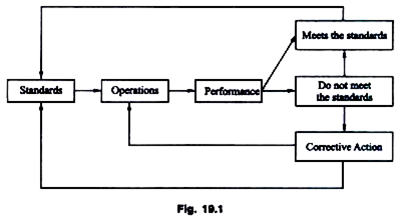
In this method, annul plans are prepared for various activities. Each plan includes setting objectives (expected results or standards), allocating resources, defining time limit, and formulating rules, policies and procedures. Annual plan control relates to sales. Periodically (mostly annually) the actual results are measured and compared with standards to judge whether annual plans are being (or have been) achieved.

Depending on the degree of difference between the planned and the actual results, causes are detected and suitable corrective actions are undertaken. Thus, it contains checking ongoing performance against annual plan and taking corrective action. Figure 1 shows five measures of annual plan control.

Measures (Evaluation Tools) of Annual Plan Control:

Following five measures are used in annual plan control:

1. Analysis of Different Sales:

Analysis of different sales contains measuring and evaluating different sales (total sales, territory- wise sales, distribution channel-wise, product-wise sales, customer-wise sales, etc.) with annual sales goals. Targets are set for different types of sales and actual sales of different categories are compared to find out how far company can achieve its sales goals.

2. Analysis of Market Share:

Here, market share is used as base for measuring, comparing, and correcting results. Market share is a proportion of company’s sales in the total sales of the industry. It helps to know how well the company is performing relative to its close competitors. Thus, the performance is assessed against expected market share and competitors’ market share.

It involves considering three types of market shares:

1. Overall market share
2. Served market share
3. Relative market share
4. Analysis of Market Expenses-to-Sales:

This type of control checks marketing expenses. It ensures that the firm is not overspending to achieve its annual sales goals. Different marketing expenses are watched in relations to sales.

Normally, company considers five components to calculate expenses-to-sales ratios and compares them with standard ratios to find out how far expenses are under control, such as:

1. Sales force-to-sales ratio
2. Advertising-to- sales ratio
3. Sales promotion-to-sales ratio
4. Marketing research-to-sales ratio
5. Sales administration-to-sales ratio

Marketing managers needs to monitor these expenses in relation to sales. If the expenses fall beyond permissible limits, it should be taken as a serious concern and needed steps are taken to keep them under control.

4. Financial Analysis:

Financial control consists of evaluating sales and sales-to-expense ratios in relation to overall financial framework. It means net profits, net sales, assets, and expenses are studied to find out rate return on total assets, and rate of return on net worth.

Financial analysis determines firm’s capacity of earnings, profits, or income. Attempts are made to find out factors influencing firm’s rate of return on net worth. Here, various ratios are calculated such as profit margin ratio (net profits + net sales), asset turnover ratio (net sales + total assets), and return on assets ratio (net profits + total assets), financial leverage (total assets + net worth) and return on net worth (net profits – net worth). Profit margin can be improved either by cutting expenses and/or increasing sales.

5. Analysis of Customer and Stakeholder Attitudes:

The measures of annual plan control discussed in former part are financial and quantitative in nature. Qualitative measures are more critical because they give early warning about what is going to happen on sales as well as profits.

Manager can initiate precautionary actions to minimize adverse impacts of forces on the future outcomes. Under this tool, customers’ attitudes are tracked to project the way they will react to the company’s offers. Alert company prefers to set up a system to monitor attitudes of customers, dealers, and other participants.

Base on their attitudes, preference and satisfaction, management can take early actions. This tool is preventive in nature as adverse impact on the future results can be prevented by advanced steps. Market- based preference scorecard analysis is used to measure (score) attitudes of customers and other participants. Such analysis reflects actual company’s performance and provides early warnings.

Measuring Customers’ Attitudes:

Here, a firm tries to measure attitudes of customers by using various methods like, complaints and suggestions, customer panels, customer survey, etc. It provides details about new customers created, existing customers lost, dissatisfied customers, relative product quality, relative service quality, target market awareness, target market preference, and other valuable information.

Measuring Stakeholders’ Attitudes:

It consists of measuring or recording stakeholders’ attitudes. It shows the pattern of stakeholders’ preference, attitudes, and overall response toward company and its offers. Stakeholders include suppliers, dealers, employees, stockholders, service providers, etc. They have critical interest and impact on company’s performance.

Without their cooperation and contribution, a company cannot realize its goals. When one or more of these stakeholders register dissatisfaction, management must take suitable actions. Methods used to track attitudes of customers can also be used for measuring attitudes of stakeholders.

Profitability Control:

In this method, the base of exercising control over marketing activities is the profitability. Certain profitability (and expenses) related standards are set and compared with actual profitability results to find out how far company is achieving profits. Profitability control calls for measuring profitability of various products, channels, territories, customer groups, order size, etc. It provides necessary information to management to determine whether products, channels, or territories should be expanded, reduced, or eliminated.

Process of Marketing-Profitability Analysis:

Systematic and logical process is used for analysis of profitability.

It involves:

1. Identifying Functional Expenses:

It consists of determining expenses to be incurred for the marketing activities like salaries, rents, advertising, selling and distribution, packing and delivery, billing and collection, etc.

2. Assigning Function Expenses to Marketing Entities:

Simply, expenses of particular head (for example, salary or advertising) are associated with different entities like products, channels, territories or customers groups.

3. Preparing Profits and Loss statement:

A profit and loss statement is prepared for each type of products, channels, territories, etc., to evaluate their relative performance. Based on relative performance in form of profitability, management can decide on products, channels or territories to be expanded, reduced or eliminated.

For example, a firm has five products, like A, B, C, D, and E. If profit and loss statement shows that:

(1) Product C is more profitable, and therefore, it must be expanded;

(2) Product B is poor, and, therefore, it must be reduced;

(3) Product D is making loss, and therefore, it must be eliminated, and

(4) Product A and product E are satisfactory, and therefore they must be maintained. In the same way, it can be applied to different territories and segments.

Table 1 shows how to prepare profit and loss statement for different products.

4. Taking Action:

On the basis of the profit and loss statement, necessary actions can be directed.

Actions include one or more of followings:

1. Expanding product(s)
2. Reducing product(s)
3. Eliminating product(s)
4. Reducing any of the expenses
5. Increasing sales, etc.

Efficiency Control:

This control, particularly, concerns with measuring spending efficiency. While profitability control reveals the relative (in relation to different entities like products, territories, channels, etc.) profits a company is earning, the efficiency control shows the ways to improve efficiency of various marketing entities like sales force, advertising, distribution, sales promotion, and so forth.

Sometimes, a post of marketing controller is created to work out a detailed programme to measure and improve efficiency of expense-centered marketing activities. Here also, in order to evaluate efficiency level of different marketing activities, the efficiency standards (of ideal performance) are set and are compared with actual performance.

Efficiency control can improve efficiency of marketing department in two ways – one is, improving ability of various marketing activities to contribute more in reaching the goals, and the second is, reducing expenses or wastage.

Types of Efficiency Control:

Figure 2 shows major types of efficiency control. Main types of efficiency control involve controlling sales force efficiency, advertising efficiency, sales promotion efficiency, distribution efficiency, and marketing research efficiency.

1. Sales Force Efficiency Control:

To measure efficiency of sale force (salesmen), certain key indicators/criteria are developed. A manager has to make a lot of calculations and paperwork.

Common criteria used to measure and evaluate the sales force efficiency include:

1. Average number of sales calls per salesman in a day
2. Average sales calls time spared per contact

iii. Average revenue generated per call

1. Average costs incurred per call
2. Entertainment cost per calls
3. Percentage of orders per specific number of calls, i.e., how many orders have been received from 100 calls made
4. Number of new customers created during specific period
5. Number of customers lost in a given period
6. Contribution of salesmen in total sales, revenue, and profits
7. Sales force costs as percentage of total sales.

Questionnaire, discussion, inspection, observation, salesman’s report, etc., methods are used for the purpose. However, most companies use salesman’s report. A unique computer-based programme or software can also be developed for speedy and accurate measurement of sales forces efficiency on a regular basis. Simply, actual performance of sales force is compared with these criteria to find out deviation, and, accordingly, necessary actions are taken.

This measurement of sales force efficiency can provide satisfactory answers of following questions:

1. What is role/contribution of sales force in selling efforts?
2. Who are the most efficient, less efficient and inefficient sales people?
3. Which are reasons responsible for poor efficiency of sales force?
4. What can/should be done to improve efficiency?
5. Advertising Efficiency Control:

Advertising is the most expensive among all the promotional tools. Major part of promotion budget is consumed by advertising alone. So, it is extremely necessary to find out efficiency level of advertising efforts. A company sets advertising goals (standards) and compared actual contribution of advertising to decide how far advertising has been capable to fulfill firm’s expectations. Advertising efficiency control mainly involves measuring cost efficiency or contribution efficiency.

Practically, it is difficult to measure the exact contribution of advertising efforts/costs. Systematic tools can be developed to measure impact of advertising qualitatively – in forms of increasing awareness, changing attitudes, and creating brand loyalty – and quantitatively – in forms of impact on sales and profits. Survey of dealers and customers can be made to collect needed data.

Common criteria used for measuring advertising efficiently include:

1. Advertising cost per thousand target customers reached by a specific media vehicle, for example, television medium.
2. Percentage of audience who read, noted, or saw message from print media.
3. Customer opinion on advertising contents and effectiveness.
4. Measurement of pre-post (before-after) advertising impact on attitudes of people toward the product.
5. Number of inquiries generated by advertising.
6. Cost per inquiry.
7. Impact of advertising on personal selling, sales promotion, public relations, publicity, and distribution.
8. Need and performance of advertising agency, etc.

Manager can compared efficiency of advertising programme with internal as well as external standards to judge comparative efficiency. He must find out causes leading to inefficiency.

One or more of following actions are initiated:

1. To changes advertising objectives and policies.
2. To change advertising message.
3. To change advertising media.
4. To change media scheduling and frequencies.
5. To change and/or train the staff.
6. To change advertising agency.
7. To change advertising budget, etc.
8. Sales Promotion Efficiency Control:

This control is exercised by sale manager. Sometimes, sales promotion manager is also appointed to deal with the issue. Sales promotion efficiency measures the impact of sales promotion efforts on sales, profits, competitiveness, and consumer satisfaction. Such efforts include offering a wide range of short-term incentives to stimulate buyer interest and consumer trial. Sales promotion is, no doubt, costly, but it seems essential. Here, manager tries to measure costs and impact of each of sales promotion tools. Normally, sales promotion tools are applied at three levels – customer level, dealer level, and sale force level.

Common criteria used for measuring sales promotion efficiency include:

1. Percentage of total sales promotion expenses to sales.
2. Costs of display, sample, coupons, and other tools per unit selling price.
3. Number of inquires generated due to display, demonstration, other such incentives.
4. Joint and individual impact of various tools on dealer interest, consumer purchase, and competitiveness.

Analysis of costs and contribution of sales promotion tools helps in selecting the most cost- effective sales promotion tools to use. A firm can reduce unnecessary costs and/or can improve contribution of each of the tools of sales promotion. It helps design suitable sales promotion strategies in term of costs, level of sales promotion, timing, and types of techniques at each of the levels.

4. Distribution Efficiency Control:

In an average, distribution costs account for 20 to 30 per cent of selling price. By a suitable distribution network, company can improve its profitability on one end and consumer satisfaction on the other end. Therefore, it is necessary to review or assess the entire distribution system periodically. Distribution efficiency control measures how far company’s distribution system is efficient to achieve marketing goals.

Common criteria used for the purpose include:

1. Percentage of total distribution costs per unit price.
2. Percentage of physical distribution (warehousing, inventory, ordering, transportation, communication, insurance, etc.) costs per unit price.
3. Percentage of channel members’ (wholesalers, retailers, agents, etc.) costs per unit price.
4. Costs and contribution of direct v/s indirect channels.
5. Potentials of using online marketing, network marketing, and by retailing chains.
6. Assessing costs of marketing channels in relation to services they offer to the company as well consumers.

Distribution efficiency gives valuable information to select the most cost-effective distribution option and sub-options. Company can minimize distribution costs and/or improve profits and competitiveness. In the same way, it can increase consumer satisfaction, too.

5. Marketing Research Efficiency Control:

Marketing research is process of gathering, analyzing, and interpreting data relating to any marketing problem. Due to dynamic nature of marketing environment, a company needs data on various relevant variables time to time. Marketing research is an expensive option. It is imperative for a firm to know how far marketing research efforts and costs are instrumental in achieving marketing goals. It provides necessary details to improve research policies and practices.

Common criteria used to measure marketing research efficiency include:

1. Annual budget of marketing research department.
2. Costs of research projects conducted in a year.
3. Effectiveness of tools and methods used for collecting and analyzing data.
4. Usefulness of findings of marketing research in decision-making.
5. Relative advantages of company’s research department v/s professional research firms, etc.

Strategic Control:

Strategic control implies a critical review of overall marketing effectiveness in relation to broad and long-term objectives and firm’s response to marketing environment. It deals with assessing firm’s ability to define and achieve marketing goals, and response pattern to environment. Normally, strategic control verifies company’s long-term performance with reference to the close competitors. Here, entire marketing system is reviewed to judge firm’s overall strengths and weaknesses. It answers the question: How far is the firm capable to exploit emerging marketing opportunities and face challenges and threats?

Methods or Tools:

As shown in Figure 3, four tools are used for strategic control – the marketing effectiveness review, the marketing audit, the marketing excellence review, and the ethical and social responsibility review. Let’s discuss each of them.

1. The Marketing Effectiveness Review:

It involves a review of overall marketing performance. It helps finding effectiveness of several business plans in term of sales growth, market share, and profitability. Attempts are made to detect causes for good-performing marketing department and poor-performing department.

Common criteria:

Some criteria are used to review marketing effectiveness.

They include:

1. Company’s Customer Philosophy:

It shows company’s approach toward customers.

1. Integrated Marketing Efforts:

It shows the way company integrates efforts of all divisions and departments for achieving marketing goals.

iii. Marketing Information:

It studies company’s policies and practices to collect, use, and disseminate critical information on a regular basis.

1. Company’s Strategic Orientation:

It shows company’s broad and long-term plans for survival and growth. It also indicates firm’s long-term plans for profits, sales, and expansion.

1. Operational Efficiency:

It shows how efficiently a company managing its current operations.

1. Public Relations Practices:

It shows company’s policies and practices to establish, maintain, and improve relations with various publics, which have direct interest in the company’s operations, and whose cooperation seems critical in achieving marketing goals.

Here, we have considered only six criteria. As per need, more criteria can be developed and used for the purpose.

A special instrument can be developed by using these criteria to measure marketing effectiveness. The instrument (a type of questionnaire or form with questions and certain number of options or intensity in each of the questions) is filled by managers of marketing and various other departments.

On the basis of this instrument, controller can calculate score of each managers of each of the departments. Level of scores received by manager or department clearly indicates the effectiveness of particular manager and/or department. Accordingly, each department is awarded class like excellent, very good, good, fair, or poor. Necessary actions can be taken on the basis of performance.

2. The Marketing Audit:

Another alternative tool for critical review of overall marketing performance is the marketing audit. Audit means to examine systematically. It is systematic examination/investigation of all critical aspects of marketing department.

Philip Kotler defines: “A marketing audit is a comprehensive, systematic, independent, and periodical examination of a company’s marketing environment, objectives, strategies, and activities with a view to determine problem areas and opportunities, and recommending a plan of action to improve the company’s marketing performance.”

Key characteristics of marketing audit have been discussed below:

1. Comprehensive:

The marketing audit covers all the major marketing activities of a business unit.

1. Systematic:

It is a systematic examination of all marketing operations. It is a well-planned and orderly task. All aspects are audited minutely. It indicates corrective actions to improve firm’s marketing performance.

iii. Independent:

Marketing audit is conducted objectively (bias-free) or neutrally. It includes self-audit, internal, or external audit. However, the external audit is considered as the best one.

1. Periodical:

The marketing audit should be conducted regularly to detect problems and avoid crisis.

1. Purposive:

Its purpose is to find out marketing problem areas and opportunities. It recommends actions to improve company’s marketing performance.

Key Issues or Decisions of Marketing Audit:

A detailed plan is prepared to conduct marketing audit.

The main decisions/issues of marketing audit include:

1. Deciding on marketing audit objectives (why).
2. Deciding on marketing audit responsibility (who).

iii. Deciding on data to be collected (what).

1. Deciding on respondents (whom).
2. Deciding on time (when and how long).
3. Deciding on areas of marketing audit (Where).

vii. Deciding on intensity of examination (How much).

viii. Deciding on methods and tools (how)

1. Deciding on audit report format
2. Deciding on actions to be taken on the basis of report.

Components of Marketing Audit:

The marketing audit examines six major components of company’s marketing operations, such as:

1. Marketing Environment Audit:

It examines impacts of micro and macro factors of marketing environment. Macro marketing environment consists of demographic, economic, environmental (ecological), technological, political and cultural factors. Micro marketing environment includes market segments, customers, competitors, dealers, suppliers, facilitators, and general public’s.

1. Marketing Strategy Audit:

It examines company’s business mission, marketing goals and objectives, resources capacity, and marketing strategies.

1. Marketing Organisation Audit:

It examines suitability of marketing organisation (structures) to implement marketing operations effectively. It includes level, relations, authority- responsibility, communication, facilities, organisation manual, etc.

1. Marketing System Audit:

It examines major systems like marketing information and research system, marketing planning system, marketing control system, new product development system, etc.

1. Marketing Productivity Audit:

It examines company’s profitability for different products, territories, and channels. It also examines cost-effectiveness for various operations.

1. Marketing Function Audit:

It examines marketing mix elements such as product, price, promotion (advertising, sales promotion, personal selling-sales force, publicity, and public relations), and distribution. For each of the components, appropriate auditing questions are designed to examine how effectively the company is performing. All relevant respondents like customers, suppliers, managers, dealers, etc., are interviewed using these questions.

Finally, the auditor prepares marketing audit report. The audit report contains individual and joint evaluation of main audit components (marketing areas). It detects strengths and weakness, and recommends actions for improving marketing performance.

3. The Marketing Excellence Review:

This is more or less similar to market effectiveness review. But, here, some excellently performing business units are taken as the base for evaluating firm’s performance. Here, performance is reviewed relatively.

The marketing excellence review is used to judge how excellently the company is performing with reference to high performing business units. A special instrument with adequate number of criteria and appropriate scaling can be developed to judge poor, good or excellent performance.

Criteria used for the purpose include:

1. Market/customer orientation
2. Market segmentation
3. Product quality
4. Quality of services
5. Approach toward competition
6. Integration and alliance
7. Approach toward dealers
8. Dealing with other stakeholders
9. Social responsibility and national services, etc.

Depending on result of the marketing excellent review, necessary actions are taken. Company’s actions mainly include undertaking all possible steps to reach the level of excellently performing business units.

4. The Ethical and Social Responsibility Review:

This review/verification decides whether firm’s marketing policies and practices are ethically and socially true. Ethics are moral principles, norms, or standards of right or wrong. Every business unit has social responsibilities toward a number of stakeholders.

In same way, marketing practices should be ethical with reference to moral norms, standards, and values. Company’s products, policies, and practices should not have adverse impact on customers, other stakeholders, and larger interest of society. Thus, here company tries to assess its ethical and social responsibility. As per need, necessary actions are taken.

Criteria used to review social and ethical responsibility include:

1. Clear definitions of illegal, immoral, and antisocial activities.
2. Company’s active efforts to practice, promote, and disseminate moral principles and to hold its employees fully responsible to observe them in practice.
3. Company’s direct contribution for social welfare of people.
4. Fulfilment of social responsibility toward various parties.
5. The adherence to all laws and regulations in force.
6. Use of business ethics in areas of product, price, promotion and distribution.

On the basis of ethical and social review, company can evaluate its performance in this regard and, if necessary, appropriate actions are taken.