Tag: OU B.com free notes

Closed economy Models

A closed economy is a country that does not import or export. A closed economy sees itself as self-sufficient and claims it does not want to trade internationally. In fact, it believes it does not need to trade.

A closed economy is a type of economy where the import and export of goods and services don’t happen, which implies that the economy is self-sufficient and has no trading activity from outside economics. The sole purpose of such an economy is to meet all the domestic consumers’ needs within the country’s border.

In a completely closed economy, there are no imports or exports. The country claims that it produces everything its citizens need. We also refer to this type economy as isolationist or an autarky.

A closed economy is the opposite of an open economy or a free-market economy. Open economies trade with other nations; they import and export goods and services. Hence, we also call them trading nations.

Maintaining a closed economy is more difficult today than two hundred years ago.

Certain raw materials are vital for the production of many products. For example, without oil, a country would not be able to function today. Many countries, such as Japan, need to import nearly all their raw materials.

Y = Cd + Id + Gd + X

Were,

Y: National income

Cd: Total domestic consumption

Id: Total investment in domestic goods and services

Gd: Government purchases of domestic goods and services

X: Exports of domestic goods and services

Importance of Closed Economy

With globalization and international trade, it is impossible to establish and maintain a closed economy. The open economy has no restrictions on imports. An open economy carries the risk of depending too much on imports. The domestic players will not be able to compete with international players. To tackle this the governments, use quotas, tariffs, and subsidies.

Resource availability across the globe varies and is never constant. Thus, depending on this availability, an international player will find out the best place to procure a particular resource and come up with the best price. Domestic players who have constraints to globalize will not be able to produce the same product at a price at par or discount compared to an international player. Thus domestic players will not be able to compete with the foreign players and the government uses the above options to provide support to domestic players and also reduce dependency on imports.

Advantages

• It is isolated from neighbors, so there is no fear of coercion or interference.
• Transit costs will be usually very less in the closed economy.
• Taxes on goods and products will be less and controlled by the government, less burden for consumers.
• Domestic players need not compete with the outside players and price competition is less.
• The self-sufficient economy will create proper demand for domestic products and agricultural products and producers will be compensated appropriately.
• Price fluctuations and volatility are easily controllable.

Limitations

• The economy will not grow if they are short of resources like oil, gas, and coal.
• The consumer will not get the best price for commodities compared to global prices.
• In case of emergencies, the economy will be hit severely as most of its production is only domestic.
• They must be able to meet all of its domestic demand internally, which is a difficult task to accomplish.
• They will have restrictions on goods and services to be sold and thus the opportunity for the consumers in such markets is more.
• Isolated economies can be looked down upon by the developing nations and globally such an economy can expect a limited aid when the need comes.

Reasons for Closed Economy

There are a few reasons a country might choose to have a closed economy or other factors that will facilitate the maintenance and building of a closed economy. It is assumed that the economy is self-sufficient and doesn’t require any import outside domestic borders to meet all of its demands from consumers.

• Isolation: An economy might be physically isolated from its trading partners (consider an island or a country surrounded by mountains). The natural boundaries of a country will factor this reason and lead the economy towards a closed one.
• Transit Cost: Due to physical isolation the transportation cost of goods will be highest leading to high transit costs. It doesn’t make sense in trade if the price of goods is increased due to the high overheads of transport and thus the economy tends to close in such cases.
• Government Decree: Governments might close down borders for taxes, regulations purposes. Thus, they will decree the trade with other economies. Violations will be punished. The government will try to support its domestic producers and tax international players to generate revenue.
• Cultural Preferences: Citizens might prefer to contact and trade only with citizens, this will lead to another barrier and facilitate a closed economy. For example, when McDonald’s came to India, people opposed the outlets claiming they use beef in their dishes and it was against culture.

Open economy Models

An open economy is a type of economy where not only domestic actors but also entities in other countries engage in trade of products (goods and services). Trade can take the form of managerial exchange, technology transfers, and all kinds of goods and services. (However, certain exceptions exist that cannot be exchanged; the railway services of a country, for example, cannot be traded with another country to avail the service.)

It contrasts with a closed economy in which international trade and finance cannot take place.

The act of selling goods or services to a foreign country is called exporting. The act of buying goods or services from a foreign country is called importing. Exporting and importing are collectively called international trade.

There are a number of economic advantages for citizens of a country with an open economy. A primary advantage is that the citizen consumers have a much larger variety of goods and services from which to choose. Additionally, consumers have an opportunity to invest their savings outside the country. There are also economic disadvantages of an open economy. Open economies are interdependent on others and this exposes them to certain unavoidable risks.

If a country has an open economy, that country’s spending in any given year need not equal its output of goods and services. A country can spend more money than it produces by borrowing from abroad, or it can spend less than it produces and lend the difference to foreigners. As of 2014 there is no totally-closed economy.

he basic model

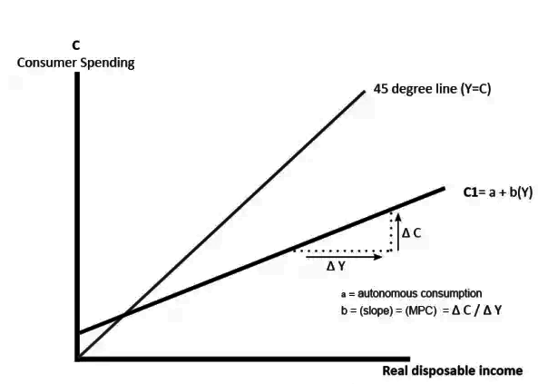
In a closed economy, all output is sold domestically, and expenditure is divided into three components: consumption, investment, and government purchases.

Y = C + I + G

where Y is the national income, C is the total consumption, I is the total investment and G is the total government expenditure. In an open economy, some output is sold domestically and some is exported to be sold abroad. We can divide expenditure on an open economy’s output Y into four components: Cd, consumption of domestic goods and services, Id, investment in domestic goods and services, Gd, government purchases of domestic goods and services, X, exports of domestic goods and services. The division of expenditure into these components is expressed in the identity

Y = Cd + Id + Gd + X.

The sum of the first three terms, Cd + I d + Gd, is domestic spending on domestic goods and services. The fourth term, X, is foreign spending on domestic goods and services (the value of exports).

Advantages

Lower Costs

Open economies are able to get cheaper imports and can sell exports at higher prices. In other words, both importers and exporters of open countries [and therefore, their consumers] benefit from price differentials.

Economic Growth

It is claimed that an open economy, with given productive resources, can have a higher GDP. Alternatively, for producing a given GDP, it spends a smaller quantity of productive resources.

This happens due to its enhanced access to improved and better technology which provides an upward thrust to economic development.

Global Prosperity and Flow of Productive Resources

Traditional economic thinking dealing with international economic transactions assumed that there was near absence of mobility (flow) of capital and other factors of production between countries.

Over time, however, the realities of international trade have belied this theory. Currently, enormous volumes of a variety of capital funds are circulating between world economies.

In addition, international flows of other inputs (raw materials and intermediate products, technology, institutional set ups, work ethos and, to some extent, even labour) have increased in varying degrees.

Some models of entrepreneurial and institutional set ups have gained the status of international standardisation. All this has also added to the overall global prosperity, as countries increasingly yearn, learn and earn together.

Superiority of Trade over Isolation

Some countries have been able to experience a rapid export-led economic growth. In contrast, it is difficult to find instances of widespread successful import substitution. Successful import substitution has been possible only in respect of a few specified industries.

Improved Availability of Goods and Services

International trade in goods and services enables each country to concentrate on the production of those goods in which it has a comparative cost advantage, and import those in which it has a comparative cost disadvantage. That way, it can add to the volume, variety and quality of goods and services that go into determining its GDP.

Impetus to Innovation

Open economies provide an incentive for research and adoption of innovations. This is because open economies have ‘lie benefit of a wider scope for their profitable application over bigger markets and recovery of huge research costs. However, being an open economy also has its drawbacks.

Disadvantages

1. Footloose Funds:

Currently, large amounts of “footloose” (that is, short term and/or speculative type) funds are moving around the world in search of places where they can be “parked” (that is, invested temporarily) within acceptable levels of safety and return.

Therefore, any change in one or both of these determining factors can lead to a large scale international movement of these funds.

2. Risk Exposure:

Open economies are interdependent. And this exposes them to certain unavoidable risks. Disturbances like trade cycles, and fluctuations in income, prices and employment etc., originating in one economy, spread to other economies also.

These disturbances may even gather strength in the process of dispersal. Consequently, all open economies, including the one from where a disturbance originates, are likely to suffer in varying degrees. Expectedly, the damage inflicted on the interdependent open economies is influenced by the following factors.

Size of the Economy:

More precisely, it is the proportion contributed by the originating economy in international economic transactions and the nature of these transactions.

By way of examples of this phenomenon, we can consider countries which have a large share in short-term capital flows or in energy sources like petroleum products, etc. and countries whose currencies are used as foreign exchange reserves, such as the US and the UK.

Intensity of the Initial Disturbance:

Other things being equal, a disturbance of higher initial intensity is likely to cause a correspondingly greater damage to the interconnected open economies.

Degree of Integration:

This factor is self-explanatory. Economies with greater restrictions on international economic transactions tend to suffer less when a disturbance originates in some other country.

When a number of South East Asian economies suffered heavily on account of a severe financial crisis in 1997-98, India could escape this disaster.

This was because Indian rupee was not freely convertible on capital account and short term capital funds could not leave the country on a large scale.

3. Indebtedness:

Large scale increase in international capital flows has resulted in problems like heavy indebtedness of certain countries and their inability to repay their debts. Starting with 1970s banks and other financial institutions, in search for better returns extended huge loans to some countries.

Their borrowers, however, could not use these loans for increasing their export earnings out of which to service them. Some of them could not “absorb” these loans productively for promoting their economic growth. This resulted in frequent bankruptcies of the borrowing governments and associated financial crises.

4. Import Dependence:

Certain varieties of imports can expose a country to undue political, economic and cultural risk. Examples are imports necessary for defence, health care, energy needs, food needs, and the like.

5. Growth Bringing Poverty:

There are instances where an expansion in international trade of a country has resulted in what is termed “immiserising growth”.

It happens when international trade adds to the productive capacity of a country, but its terms of trade deteriorate so much that there is a net decline in its economic welfare.

In addition, it is also possible that while there is an overall increase in economic welfare of the country, some sections happen to be net losers.

6. Constraints on Resource Use:

It is possible that a country is forced to adopt certain production technologies which do not let it make an optimum use of its factor-endowment.

Alternatively, it may have to face restrictions on its exports. Such a state of affairs may be thrust upon a country which has a weak bargaining strength or which is facing balance of payments difficulties.

For example, the USA and several other industrially advanced countries (with abundant capital resources) are interested in weakening competition from imported goods from labour-surplus countries like India.

They are insisting that imports should be totally banned (or at least severely restricted) if they are produced by “exploited” or “sweat” labour (that is, by labour which is paid at rates lower than those in rich countries like the USA) or by child labour.

The flaws in this logic are quite easy to see. Wage rates are expected to be lower in a labour-surplus economy. And it is this fact which makes its labour-intensive products competitive.

Similarly, it is a fact that child labour is extensively used in India in the manufacture of carpets and other handicrafts.

It is also admitted that it would be better if these children, instead of working, were attending schools. But that happy situation can be attained only if our economy grows and income levels of the parents rise. Till then, if these children are prevented from taking up jobs, their families would become still poorer.

7. Problems of Foreign Exchange:

These days, currencies are on “paper standard”.’ And historically, some leading currencies of the world (the most prominent being the US dollar) are being held as “foreign exchange reserves” by countries of the world for financing their trade and other international economic transactions.

Moreover, a rapid expansion in these transactions has added to the need for ever-increasing volumes of foreign exchange reserves.

The gross national income (GNI), previously known as gross national product (GNP), is the total domestic and foreign output claimed by residents of a country, consisting of gross domestic product (GDP), plus factor incomes earned by foreign residents, minus income earned in the domestic economy by non-residents.

GNI is the total amount of money earned by a nation’s people and businesses. It is used to measure and track a nation’s wealth from year to year. The number includes the nation’s gross domestic product plus the income it receives from overseas sources.

GNI is an alternative to gross domestic product (GDP) as a means of measuring and tracking a nation’s wealth and is considered a more accurate indicator for some nations.

Gross national product (GNP) is the market value of all the goods and services produced in one year by labor and property supplied by the citizens of a country. Unlike gross domestic product (GDP), which defines production based on the geographical location of production, GNP indicates allocated production based on location of ownership. In fact it calculates income by the location of ownership and residence, and so its name is also the less ambiguous gross national income.

GNP is an economic statistic that is equal to GDP plus any income earned by residents from overseas investments minus income earned within the domestic economy by overseas residents.

GNP does not distinguish between qualitative improvements in the state of the technical arts (e.g., increasing computer processing speeds), and quantitative increases in goods (e.g., number of computers produced), and considers both to be forms of “economic growth”.

The term gross national income (GNI) has gradually replaced the Gross national product (GNP) in international statistics. While being conceptually identical, the precise calculation method has evolved at the same time as the name change.

Criticism of gross national product

The gross national product (GNP) measures the welfare of a nation’s economy through the aggregate of products and services produced in that nation. Although GNP is a proficient measurement of the magnitude of the economy, many economists, environmentalists and citizens have been arguing the validity of the GNP in respect to measuring welfare.

Joseph Stiglitz, Nobel Prize–winning economist, states that this standard measurement for any national economy has become deficient as a measure of long-term economic health in our recently resource-driven and globalizing world. Critics suggest that GNP often includes the environment on the wrong side of the balance sheet because if someone first pollutes and then another person cleans the pollution, both activities add to GNP making environmental degradation frequently look good for the economy.

Critics of mainstream economics complain that GNP compiles spending that makes us worse off, spending that allows us to stay in the same place, and spending that makes us better off all in a single measure, giving a nation no clue if they are making progress or not.

Manfred Max-Neef, Chilean economist, explains that politicians feel that it is irrelevant whether the spending is productive, unproductive, or destructive. In this sense, it is common to see political policies that call to depredate a natural resource in order to increase the GNP. To take into account the environmental depredation and resource depletion, there is a call to shift away from the traditional GNP and construct an assessment of national product that takes into account environmental effects.

Need

Many people are calling for a green national product that would indicate if activities benefit or harm the economy and well-being. This green national product would revolve around the social and economic issues on which many green movements have focused: care for the earth and all that sustain it. This new national product would differ from the traditional GNP by addressing both the sustainability and well-being of the planet and its inhabitants. It is essential that this system takes into account natural capital, which is currently hidden from our traditional measurement.

Green GNP

Is an economic and environmental accounting framework which measures the national wealth by accounting for exhaustion of natural resources and degradation of environment and investment in environment support.

The goal of Green GDP is one of the dreams of every economist. An economist who could actually come up with a serious theory of Green GDP would go down in history as the one of the greatest economists ever!

That’s because in the big picture, “externalities” costs or benefits which are not born by the person performing the economic action which causes them are very important in determining the wealth of a society. But economists are very limited in their ability to study them.

Externalities include things like the cost imposed on society by potentially harmful emissions into the common spaces.

But Green GDP is cheap ideological political propaganda masquerading as economic science.

As economics, it is pure rubbish. It manufactures silly economic cost estimates with absolutely no scientific basis, based purely on continually changing “narratives”, invented by activists, and kept alive (as people eventually discover that their predictions are all falsified by reality) by

(a) Altering the public record of what they were saying

(b) Emotionalist propaganda to appeal to those who lack the intellectual curiosity to find out the facts. All this solely to support the authoritarian political agenda of its promoters.

In economics, the consumption function describes a relationship between consumption and disposable income. The concept is believed to have been introduced into macroeconomics by John Maynard Keynes in 1936, who used it to develop the notion of a government spending multiplier.

The Keynesian consumption function expresses the level of consumer spending depending on three factors.

• Yd = disposable income (income after government intervention – e.g. benefits, and taxes)
• a = autonomous consumption (consumption when income is zero. e.g. even with no income, you may borrow to be able to buy food)
• b = marginal propensity to consume (the % of extra income that is spent). Also known as induced consumption.

Consumption function formula

    C = a + b Yd

This suggests consumption is primarily determined by the level of disposable income (Yd). Higher Yd leads to higher consumer spending.

This model suggests that as income rises, consumer spending will rise. However, spending will increase at a lower rate than income.

• At low incomes, people will spend a high proportion of their income. The average propensity to consume could be one or greater than one. This means people spend everything they have. When you have low income, you don’t have the luxury of being able to save. You need to spend everything you have on essentials.
• However, as incomes rise, people can afford the luxury of saving a higher proportion of their income. Therefore, as incomes rise, spending increases at a lower rate than disposable income. People with high incomes have a lower average propensity to spend.

Limitations of consumption function

• Life cycle factors, Students more likely to borrow and spend during university days.
• Behavioural factors, People may be influenced by general optimism.

importance of the concept of propensity to consume is that we derive the theory of multiplier from it which has great practical importance in the formulation of macro-economic policy, especially of public works in times of depression. The magnitude of multiplier is equal to the reciprocal of one minus marginal propensity to consume (K = 1/1-MPC) where K stands for multiplier and MPC for marginal propensity to consume. According to this concept of multiplier, when investment increases, in­come, output and employment increase by a multiple amount, depending upon the size of the multiplier.

Income increases manifold than the original investment because of the nature of consumption function. When some investment in some projects is undertaken, it leads to the increase in income of those employed in the projects but the process does not stop here.

The increases in income are further spent on consumption and this leads to further increase in income and so the chain of increases in income and consumption continues and the ultimate increase in income and employment is multiple of the original increment in investment.

If the marginal propensity to consume were equal to zero, then all increments in income brought about by additional investment would have been saved and therefore multiplier process would not have worked. Since the marginal propensity to consume is greater than zero, the increase in net investment has a multiplier effect on income, output and employment. Thus, the effect of investment on income depends on the size of the multiplier which depends on the value of the marginal propensity to consume. The greater the marginal propensity to consume, the greater the size of the multiplier.

(4) From the concept of consumption function, we can also explain why there is a tendency for the marginal efficiency of capital to decline. The declining tendency of the marginal effi­ciency of capital is due to the nature of the consumption function. Two features of consumption function are important. First, the marginal propensity to consume is less than one which implies that as income increases, consumption increases less than this. Secondly, consumption function is stable in the short run i.e., it does not shift much in the short run.

As we know that the level of investment is a crucial factor in the determination of income and employment, fluctuations in the levels of income and employment depend primarily on the fluctuations in investment. The investment demand in the short run is determined by the rate of interest on the one hand and marginal efficiency of capital on the other. Since the rate of interest is relatively sticky, it is the marginal efficiency of capital which greatly affects the level of investment in the short run.

Marginal efficiency of capital is nothing but the expected rate of profit on investment in the future. Thus, the marginal efficiency of capital is determined by the expectations of the entrepreneurs regarding the earning of profits from capital assets in the future.

Now, the most, important fact that affects the entrepreneurs expectations regarding profit prospects and thereby the marginal efficiency of capital is the level of future consumption demand for goods and services. Their estimate of future consumption demand depends on, among others, on the population growth. If population growth of a country is expected to fall as was estimated in the early thirties when Keynes wrote his book (General Theory of Employment, Interest and Money), this would adversely affect future consumption demand which in turn would adversely affect investment in the long run, Besides, according to Keynes, average propensity to consume (APC) falls as income of a community increases overtime.

This also adversely affects inducement to invest. If there does not occur capital-using technological change, this will result in decline in investment opportunities in the long run, causing secular stagnation. Thus, we see that in the Keynesian scheme of things level of investment depends upon the level of consumption demand in the long run.

Since marginal propensity to consume is less than one and also the consumption function is stable when income increases, consumption does not increase proportionately. As a result, the aggregate demand becomes deficient and the marginal efficiency of capital declines. The decline in the marginal efficiency of capital adversely affects investment which stops rising. As a result, the growth process stops and economic recession occurs.

In this way, Keynes himself and later important Keynesian economist, Prof. A.H. Hansen developed the theory of secular stagnation for the mature capitalist economies. This secular stagnation theory is based upon the assertion that investment opportunities in a capitalist economy will be exhausted soon due to the absence of the possibilities of increasing consumption demand. The meagre possibilities of increasing investment in the mature capitalist economies, according to them, were partly due to the constancy of consumption function and declining average propensity to consume which caused the marginal efficiency of capital to decline.

Theory of secular stagnation has not been found true by empirical evidence in the last over seventy years of growth in the capitalist developed countries. However, the fact that current consumption is influenced by changes in rate of interest, stock of wealth and price level and further that it is the changes current consumption level that determine short-run business expectations about future yields from investment which cause fluctuations in investment.

Together with the working of multiplier fluctuations in investment cause business cycles in a free market economy. This shows the great importance of Keynes’s consumption function and the factors that determine it.

Investment function

The investment function is a summary of the variables that influence the levels of aggregate investments.

The level of income, output and employment in an economy depends upon effective demand, which in turn, depends upon expenditures on consumption goods and investment goods (Y = C + I).

Consumption depends upon the propensity to consume, which, we have learnt, in more or less stable in the short period and is less than unity. Greater reliance, therefore, has to be placed on the other constituent (investment) of income.

The reason for investment being inversely related to the Interest rate is simply because the interest rate is a measure of the opportunity cost of those resources. If the resources instead of financing the investment could be invested in financial assets, there is an opportunity cost of (1+r), where r is the interest rate. This implies higher investment spending with a lower interest rate. When GDP increases, the output and the capacity utilization increases. This results in an increase of capital investment. At last, a higher Tobins q is represented when the market puts a high value of the installed capital and buys stocks in the firm for a higher price. The firm can then raise more resources per share issued and increase their investments.

Out of the two components (consumption and investment) of income, consumption being stable, fluctuations in effective demand (income) are to be traced through fluctuations in investment. Investment, thus, comes to play a strategic role in determining the level of income, output and employment at a time.

We can establish the importance of investment in another way also. In order to maintain an equilibrium level of income (Y = C + I), consumption expenditures plus investment expenditures must equal the total income (Y); but according to Psychological Law of Consumption given by Keynes, as income increases consumption also increases but by less than the increment in income. This means that a part of the increment in income is not spent but saved.

The savings must be invested to bridge the gap between an increase in income and consumption. If this gap is not plugged by an increase in investment expenditures, the result would be an unintended increase in the stocks of goods (inventories), which in turn, would lead to depression and mass unemployment. Hence, investment rules the roost. In Keynesian economics investment means real investment i.e., investment in the building of new machines, new factory buildings, roads, bridges and other forms of productive capital stock of the community, including increase in inventories.

Types of Investment:

1. Induced Investment:

Real investment may be induced. Induced investment is profit or income motivated. Factors like prices, wages and interest changes which affect profits influence induced investment. Similarly demand also influences it. When income increases, consumption de­mand also increases and to meet this, investment increases. In the ultimate analysis, induced investment is a function of in­come i.e., I = f(Y). It is income elastic. It increases or de­creases with the rise or fall in income, as shown in Figure 1.

Induced Investment

is the investment curve which shows induced invest­ment at various levels of income. Induced investment is zero at OY1 income. When income rises to OY3 induced investment is I3Yy A fall in income to OY2 also reduces induced investment to I2Y2.

Induced investment may be further divided into (i) the average propensity to invest, and (ii) the marginal propensity to invest:

(i) The average propensity to invest is the ratio of investment to income, I/Y. If the income is Rs. 40 crores and investment is Rs. 4 crores, I/Y = 4/40 = 0.1. In terms of the above figure, the average propensity to invest at OY3 income level is I3Y3/ OY3

(ii) The marginal propensity to invest is the ratio of change in investment to the change in income, i.e., clip_image004I/clip_image004[1]Y. If the change in investment, I=Rs 2 crores and the change in income, Y = Rs 10 crores, I/∆Y = 2/10=0.2

2. Autonomous Investment:

Autonomous investment is independent of the level of income and is thus income inelastic. It is influenced by exogenous factors like innovations, inventions, growth of population and labour force, researches, social and legal institutions, weather changes, war, revolution, etc. But it is not influenced by changes in demand. Rather, it influ­ences the demand. Investment in economic and social overheads whether made by the government or the private enterprise is au­tonomous.

Such investment includes expenditure on building, dams, roads, canals, schools, hospitals, etc. Since investment on these projects is generally associated with public policy, autonomous in­vestment is regarded as public investment. In the long-run, private investment of all types may be autonomous because it is influenced by exogenous factors. Diagrammatically, autonomous investment is shown as a curve parallel to the horizontal axis as I1I’ curve in Figure 2. It indicates that at all levels of income, the amount of investment OI1 remains constant.

Autonomous Investment

The upward shift of the curve to I2I” indicates an increased steady flow of investment at a constant rate OI2 at various levels of income. However, for purposes of income determination, the autonomous investment curve is superimposed on the С curve in a 45° line diagram.

3. Determinants of the Level of Investment:

The decision to invest in a new capital asset depends on whether the expected rate of return on the new investment is equal to or greater or less than the rate of interest to be paid on the funds needed to purchase this asset. It is only when the expected rate of return is higher than the interest rate that investment will be made in acquiring new capital assets.

In reality, there are three factors that are taken into consideration while making any investment decision. They are the cost of the capital asset, the expected rate of return from it during its lifetime, and the market rate of interest. Keynes sums up these factors in his concept of the marginal efficiency of capital (MEC).

The Keynesian Multiplier is an economic theory that asserts that an increase in private consumption expenditure, investment expenditure, or net government spending (gross government spending government tax revenue) raises the total Gross Domestic Product (GDP) by more than the amount of the increase. Therefore, if private consumption expenditure increases by 10 units, the total GDP will increase by more than 10 units.

Components of the Keynesian Theory

The three main components of the Keynesian Theory are:

• Aggregate demand is influenced by the decisions in the private and public sector. The level of demand by the private sector could exert an effect on macroeconomic conditions. For example, a decrease in aggregate spending can bring the economy into a recession. However, the negative impact of private decision-making can be mitigated through government intervention with a fiscal or monetary stimulus.
• Prices such as wages are often slow to respond to changes in demand and supply. It is why there are many instances of a shortage or an excess in the supply of labor.
• A change in aggregate demand causes the greatest impact on the output and employment in the economy. Keynesian economic theory says that spending by consumers and the government, investment, and exports will increase the level of output. Even a change in one the components will cause total output to change.

Calculating the Keynesian Multiplier

The value of the multiplier depends on the marginal propensity to consume and the marginal propensity to save.

1. Marginal Propensity to Save

The change in total savings as a result of a change in total income is known as the marginal propensity to save. When an individual’s income increases, the marginal propensity to save (MPS) measures the proportion of income the person saves rather than spend on goods and services. It is calculated as MPS = ΔS / ΔY.

2. Marginal Propensity to Consume

The change in total consumption as a result of a change in total income is known as the marginal propensity to consume. The marginal propensity to consume (MPC) measures how consumer spending changes with a change in income. Using the figures above, the MPC is ΔC / ΔY = 300/600 = 0.5.

Leakages in the Multiplier Process:

We have seen above that as a result of increase in investment, the level of income increases by a multiple of it. In our above analysis, saving is a leakage in the multiplier process. Had there been no saving and as a result marginal propensity to consume were equal to 1, the multiplier would have been equal to infinity.

In that case as a result of some initial increase in investment, income would go on rising indefinitely. Since marginal propensity to consume is actually less than one, some saving does take place. Therefore, multiplier in actual practice is less than infinity.

But besides saving, there are other leakages in the process of income generation which reduce the size of the multiplier. Therefore, the increase in income as a result of some increase in investment will be less than warranted by the size of the multiplier measured by the given marginal propensity to consume. We explain below the various leakages that occur in the income stream and reduce the size of multiplier in the real world.

Paying off debts:

The first leakage in the multiplier process occurs in the form of payment of debts by the people, especially by businessmen. In the real world, all income received by the people as a result of some increase in investment is not consumed. A part of the increment in income is used for paying back the debts which the people have taken from moneylenders, banks or other financial institutions.

The incomes used for paying back the debts do not get spent on consumer goods and services and therefore leak away from the income stream. This reduces the size of the multiplier. Of course, when incomes received by the moneylenders, banks or institutions are again lent back to the people, they come back to the income stream and enhance the size of multiplier. But this may or may not happen.

Holding of idle cash balances:

If the people hold apart of their increment in income as idle cash balances and do not use it for consumption, they also constitute leakage in the multiplier process. As we have seen, people keep part of their income for satisfying their precautionary and speculative motives, money kept for such purposes is not consumed and therefore does not appear in the successive rounds of consumption expenditure and therefore reduces the increments in total income and output.

Imports:

In our above analysis of the working of the multiplier process we have taken the example of a closed economy, that is, an economy with no foreign trade. If it is an open economy as is usually the case, then a part of increment in income will also be spent on the imports of consumer goods. The proportion of increments in income spent on the imports of consumer goods will generate income in other countries and will not help in raising income and output in the domestic economy.

Increase in Prices:

Price inflation constitutes another important leakage in the working of the multiplier process in real terms. The multiplier works in real terms only when as a result of increase in money income and aggregate demand, output of consumer goods is also increased.

When output of consumer goods cannot be easily increased, a part of the increases in the money income and aggregate demand raises prices of the goods rather than their output. Therefore, the multiplier is reduced to the extent of price inflation. In developing countries like India the extra incomes and demand are mostly spent on food-grains whose output cannot be increased so easily.

Therefore, the increments in demand raise the prices of goods to a greater extent than the increase in their output. Besides, in developing countries like India, there is not much excess capacity in many consumer goods industries, especially in agriculture and other wage-goods industries.

Therefore, when income and demand increase as a result of increase in investment, it generally raises the prices of these goods rather than their output and therefore weakens the working of the multiplier in real terms. Thus, it was often asserted in the past that Keynesian theory of multiplier was not very much relevant to the conditions of developing countries like India. However, we shall discuss later that this old view about the working of Keynes’ multiplier is not fully correct.

The above various leakages reduce the multiplier effect of the investment undertaken. If these leakages are plugged, the effect of change in investment on income and employment would be greater.

Multiplier with Changes in Price Level:

In our above analysis of multiplier with aggregate demand curve, it is assumed that price level remains constant and the firms are willing to supply more output at a given price. How much national income or GNP increases as a result of any autonomous expenditure such as government expenditure, investment expenditure, net exports is determined by a shift in aggregate demand curve by the size of simple Keynesian multiplier when price level is fixed.

This implies a horizontal short-run supply curve. However, as studied above, short-run aggregate supply curve slopes upward as the firms are willing to supply additional output in the short run only at a higher price level. With short-run aggregate supply curve sloping upward, a rightward shift in aggregate demand curve raises new equilibrium GNP level not equal to the horizontal shift in the aggregate demand curve but less than it.

Consequently, the size of multiplier is smaller than that of simple Keynesian multiplier with a given fixed price level. This is because a part of expansionary effect of GNP of the increase in autonomous government expenditure is offset by rise in the price level.

The multiplier effect in case of upward sloping curve is shown in Fig. 10.3. To begin with, in the top panel of Fig. 10.3 aggregate expenditure curve AE₀ intersects 45° line at point Sand determines Y₀ equilibrium level of GNP. In the panel at the bottom of Fig. 10.3 the corresponding aggregate demand curve AD₀ and the short-run aggregate supply curve SAS intersect at B’ at the above determined GNP level K₀. Now suppose autonomous investment expenditure (which is independent of changes in price level) increases by AI.

As a result, aggregate expenditure curve AE shifts upward to AE₁ and determines new equilibrium GNP level equal to Y₂. In the lower panel (b), due to the upward shift in aggregate expenditure curve, aggregate demand curve shifts rightward from AD to AD₁The horizontal shift in the aggregate demand curve at a given price level is determined by the increase in aggregate expenditure multiplied by the simple Keynesian multiplier at the given fixed price level (B’H or ∆Y = ∆I 1/1- MPC) But given the upward sloping short-run aggregate supply curve SAS with new aggregate demand curve AD₁, price level does not remain fixed. As will be seen from the lower panel (b) of Fig. 10.3, the aggregate demand curve AD₁ intersects the short-run aggregate supply curve SAS at point R’ and as a result price level rises to P₁.

Now, with this rise in price level to P₁, aggregate expenditure curve in the upper panel (a) will not remain unaffected but will shift downward. This fall in aggregate expenditure curve is due to the adverse effects on wealth or real balances, interest rate and net exports. Much of wealth is held in the form of bank deposits, bonds and shares of companies and other assets.

With the rise in price level, real value or purchasing power of wealth possessed by the people declines. This induces them to spend less. As a result, consumption expenditure declines due to this wealth effect. Secondly, the rise in price level reduces the supply of real money balances (M^s/P) that causes a shift in money supply curve to the left.

Given the demand function for money (M^d), the decline in the real money supply will cause rate of interest to rise. Now, the rise in interest will induce private investment expenditure to decline. Lastly, rise in price level in the domestic economy will adversely affect exports of a country causing net exports to fall.

Thus, as a result of negative effects of rise in price level on real wealth, private investment and net exports, in the upper panel (a) of Fig. 10.3 aggregate expenditure curve shifts downward to AE₁ (dotted) so that it determines GNP level Y₁ at which aggregate expenditure curve AE₁ intersects 45° line. This also corresponds to the intersection of aggregate demand curve AD₁ and short-run aggregate supply curve SAS point R’ in the lower panel (b) of Q 1. Fig. 10.3.

Thus with the upward sloping short-run aggregate supply curve SAS, the effect of increase in autonomous investment expenditure (or for that matter increase in any other autonomous expenditure such as Government expenditure, net exports, autonomous consumption) on the GNP level can be visualized to occur in two stages.

First, increase in investment expenditure shifts aggregate expenditure curve AE upward in the upper panel (a) of Fig. 10.3 and correspondingly aggregate demand curve in the lower panel (b) shifts to the right to AD₁ and brings about increase in GNP level from Y₀ to Y₂with the given fixed price level P_r In the second stage due to the upward sloping short-run aggregate supply curve SAS, the rightward shift in the aggregate demand curve causes price level to rise from P₀ to P_t and causes decrease in GNP from Y₂to Y₁

However, as shall be seen from Fig. 10.3, when price level effect is taken into account, the increase in investment expenditure has still a multiplier effect on real GDP but this effect is smaller than it would be if price level remained fixed. It may be further noted that steeper the slope of the short- run supply curve, the greater is the increase in the price level and smaller is the effect on real GNP.

Importance of the Concept of Multiplier:

Multiplier is one of the most important concepts developed by J.M. Keynes to explain the determination of income and employment in an economy. The theory of multiplier has been used to explain the cumulative upward and downward swings of the trade cycles that occur in a free-enterprise capitalist economy. When investment in an economy rises, it has a multiple and cumulative effect on national income, output and employment.

As a result, economy experiences rapid upward movement. On the other hand, when due to some reasons, especially due to the adverse change in the expectations of the business class, investment falls, then backward working of the multiplier causes a multiple and cumulative fall in income, output and employment and as a result the economy rapidly moves on downswing of the trade cycle. Thus, Keynesian theory of multiplier helps a good deal in explaining the movements of trade cycles or fluctuations in the economy.

The theory of multiplier has also a great practical importance in the field of fiscal policy to be pursued by the Government to get out of the depression and achieve the state of full employment. To get rid of depression and remove unemployment, Government investment in public works was recommended even before Keynes.

But it was thought that the increase in income will be limited to the amount of investment undertaken in these public works. But the importance of public works is enhanced when it is realised that the total effect on income, output and employment as a result of some initial investment has a multiplier effect. Thus, Keynes recommended Government investment in public works to solve the problem of depression and unemployment.

The public investment in public works such as road building, construction of hospitals, schools, irrigation facilities will raise aggregate demand by a multiple amount. The multiple increase in income and demand will also encourage the increase in private investment.

Thus, the deficiency in private investment which leads to the state of depression and underemployment equilibrium will now be made up and a state of full employment will be restored. If the multiplier had not worked, the income and demand would have risen as a result of some public investment but not as much as they rise with the multiplier effect.

Inspired by the Keynesian theory of multiplier, expansionary fiscal policy of increase in Government expenditure and reduction in income tax have been adopted by President John Kennedy and President George W. Bush in the United States of America to remove involuntary unemployment and depression. This had a great success in removing unemployment and depression and therefore, Keynesian theory of multiplier was vindicated and as a result people’s belief in it increased.

Net National Product is the market value of all final goods and services after allowing for depreciation. It is also called National Income at market price. When charges for depreciation are deducted from the gross national product.

Net national product (NNP) refers to gross national product (GNP), i.e., the total market value of all final goods and services produced by the factors of production of a country or other polity during a given time period, minus depreciation. Similarly, net domestic product (NDP) corresponds to gross domestic product (GDP) minus depreciation. Depreciation describes the devaluation of fixed capital through wear and tear associated with its use in productive activities.

Closely related to the concept of GNP is another concept called NNP of a country. NNP is a more accurate measure of total value of goods and services by a country. It is derived from GNP figures. As a rough estimate, GNP is very useful indicator of total production of a country. But if we are interested to have an accurate and true measure of what a country is producing and what is available for uses, then GNP has a serious defect.

In national accounting, net national product (NNP) and net domestic product (NDP) are given by the two following formulas:

NNP=GNP-Depreciation

NDP=GDP-Depreciation

Anyway, to measure NNP, we must make a distinction between gross investment (IG) and net investment (IN). Gross investment refers to total expenditure for new plant, equipment, etc., plus the change in inventories. Net investment is equal to gross investment less depreciation.

That is,

IN = IG – depreciation

Since, GNP = C + IG + G + (X – M),

NNP = C + IN + G + (X – M)

Or, NNP = GNP – depreciation

Although NNP gives us the better measure of an economy’s performance, we pay more attention to GNP. This is because estimation of NNP is difficult in practice, as one has to measure depreciation to obtain the net investment figure. In practice, GNP is the more commonly used indicator than NNP.

Importance of the NNP

To many of us, the net national product may seem an insignificant figure another number among the many items discussed by economists. However, we will be mistaken to not understand the importance and significance it represents in our daily lives.

A vibrant economy, represented in part by the NNP, can help us to decide if a particular country is worth moving to or if the economy is growing at a pace that we feel comfortable being paid in the local currency. Thus, the NNP can be a useful figure to understand and interpret, especially when making comparisons among locales.

Sustainability and the NNP

Environmental sustainability is a topic that concerns us all as global citizens. It’s been suggested that the net national product depreciation includes an element that accounts for natural resource and environmental depreciation. It will help measure the true impact of certain types of growth on the country, including what can be considered environmental assets. Forestry, mining, and toxic fumes will all weigh down on the NNP and can provide a more long-term view of a company’s strategic growth strategy.

The measurement of environmental impacts when calculating a countries NNP can be considered controversial. Difficulties will no doubt arise when attempting to create a precise measurement in determining how much depreciation the extraction of raw materials should account for.

While precise measurements will be difficult to gain a consensus around, measuring the environmental impacts and being aware of production methods are important factors to consider when balancing the protection of the environment, while also ensuring economic growth.

Economic Welfare

Before knowing the relation between economic welfare and national income, it is essential to define economic welfare. ‘Welfare’ is a state of the mind which reflects human happiness and satisfaction. In actuality, welfare is a happy state of human mind.

Pigou regards individual welfare as the sum total of all satisfactions experienced by an individual and social welfare as the sum total of individual welfares. He divides welfare into economic welfare and non-economic welfare. Economic Welfare is that part of social welfare which can directly or indirectly be measured in money.

Pigou attaches great importance to economic welfare because welfare is a very wide term. In his words: “The range of our enquiry becomes restricted to that part of social(general) welfare that can be brought directly or indirectly into relation with the measuring rod of money.’” On the contrary, non-economic welfare is that part of social welfare which cannot be measured in money, for instance moral welfare.

But it is not proper to differentiate between economic and non-economic welfare on the basis of money. Pigou also accepts it. According to him, non-economic welfare can be improved upon in two ways. First, by the income-earning method. Longer hours of working and unfavourable conditions will affect economic welfare adversely. Second, by the income-spending method.

It is assumed in economic welfare that expenditures incurred on different consumption goods provide the same amount of satisfaction. But in actuality it is not so, because when the utility of purchased goods starts diminishing the non-economic welfare declines which results in reducing the total welfare. But Pigou is of the view that it is not possible to calculate such effects, because non-economic welfare cannot be measured in terms of money.

The economist should, therefore, proceed with the assumption that the effect of economic causes on economic welfare applies also to total welfare. Hence, Pigou arrives at the conclusion that the increase in economic welfare results in the increase of total welfare and vice versa.

But it is not possible always, because the causes that lead to an increase in economic welfare may also reduce non-economic welfare. The increase in total welfare may, therefore, be less than anticipated. For instance, with the increase in income, both the economic welfare and total welfare increase and vice versa.

But economic welfare depends not only on the amount of income but also on the methods of earning and spending it. When the workers earn more by working in factories but reside in slums and vitiated atmosphere, the total welfare cannot be said to have increased, even though the economic welfare might have increased.

To obtain MEW, GNP totals are adjusted by:

(1) Reclassifi­cation of GNP expenditure into C, I and intermediate production, where only C contributes to current economic welfare,

(2) Imputations of the value of services of consumer capital, the value of leisure and the value of household work, and

(3) A negative correction for some of the dis-amenities of urbanization. Paul Samuelson called it net economic welfare.

Relationship

The effect of national income can be studied in two ways.

1. Change in the size of National Income
2. Changes in Distribution of National Income

Change in the Size of National Income:

The change in the size of national income may be positive or negative. The positive change in the national income increases its volume. As a result, people consume more of goods and services, which lead to increase in the economic welfare.

Whereas the negative change in national income results in reduction of its volume. People get lesser goods and services for consumption which leads to decrease in economic welfare. But this relationship depends on a number of factors.

1. Change in Prices:

Is the change in national income real or monetary? If the change in national income is due to change in prices, it will be difficult to measure the real change in economic welfare. For example, when the national income increases as a result of increase in prices, the increase in economic welfare is not possible because it is probable that the output of goods and services may not have increased. It is more likely that the economic welfare would decline as a result of increase in prices. It is only the real increase in national income that increases economic welfare.

2. Per Capita Income:

National income cannot be a reliable index of economic welfare, if per capita income is not kept in mind. It is possible that with the increase in national income, the population may increase at the same pace and thus the per capita income may not increase at all.

In such a situation, the increase in national income will not result in increase in economic welfare. But from this, it should not be concluded that the increase in national income results in increase in economic welfare and vice versa.

It is possible that as a result of increase in national income, the per capita income might have risen. But if the national income has increased due to the production of capital goods and there is shortage of consumption goods on account of decrease in their output, the economic welfare will not increase even if the national income and per capita income rise.

This is because the economic welfare of people depends not on capital goods but on consumption goods used by them. Similarly, when the national income and the per capita income rise sharply during war time, the economic welfare does not increase because during war days the entire production capacity of the country is engaged in producing war material and there is shortage of consumption goods. As a result, the standard of living of the people fall and the economic welfare decreases.

Often, even with the increase in national income and per capita income the economic welfare decreases. This is the case when as a result of the increase in national income, income of the richer sections of the society increases and the poor do not gain at all from it. In other words, the rich become richer and the poor become poorer. Thus, when the economic welfare of the rich increases and that of the poor decreases, the total economic welfare decreases.

3. Working Conditions:

It depends on the manner in which the increase in national income comes about. The economic welfare cannot be said to have increased, if the increase in national income is due to exploitation of labour e.g., increase in production by workers working for longer hours, by paying them lesser wages than the minimum. Forcing them to put their women and children to work, by not providing them with facilities of transport to and from the factories and of residence, and their residing in slums.

4. Method of Spending:

The influence of increase in national income on economic welfare depends also on the method of spending adopted by the people. If with the increase in income, people spend on such necessities and facilities as milk, ghee, eggs, fans, etc. which increase efficiency, the economic welfare will increase.

But on the contrary, the expenditure on drinking, gambling etc. will result in decreasing the economic welfare. As a matter of fact, the increase or decrease in economic welfare as a result of increase in national income depends on changes in the tastes of people. If the change in fashions and tastes takes place in the direction of the consumption of better goods, the economic welfare increases.

Changes in Distribution of National Income:

1. Transfer of Wealth from the Rich to the Poor:

The redistribution of wealth in favour of the poor is brought about by reducing the wealth of the rich and increasing the income of the poor. The income of the richer sections can be reduced by adopting a number of measures, e.g., by progressive taxation on income, property etc., by imposing checks on monopoly, by nationalising social services, by levying duties on costly and foreign goods which are used by the rich and so on.

On the other hand, the income of the poor can also be raised in a number of ways, e.g., by fixing a minimum wage rate, by increasing the production of goods used by the poor, by fixing the prices of such goods, by granting financial assistance to the producers of these goods, by the distribution of goods through co-operative stores, and by providing free education, social security and low rent accommodation to the poor. When the distribution of income takes place in favour of the poor through these methods, the economic welfare increases.

But it is not essential that the equal distribution of national income would lead to increase in economic welfare. On the contrary, there is a greater possibility of economic welfare decreasing if the policy towards the rich is not rational. Heavy taxation and progressive taxes at high rates affect adversely the productive capacity, investment and capital formation, thereby decreasing the national income.

Similarly, when through the efforts of the government, the income of the poor increases but if they spend that income on bad goods like drinking, gambling etc. or if their population increases, the economic welfare will decrease.

Both these situations are not real and only express the fears, because the government, while imposing different kinds of progressive taxes on the rich, keeps particularly in view that taxation should not affect the production and investment adversely. On the other hand, when the income of a poor man increases, he tries to provide better education to his children and to improve his standard of living, his welfare increases.

2. By Transfer of Wealth from the Poor to the Rich:

When as a result of increase in national income, the transfer of wealth takes place in the former manner, the economic welfare decreases. This happens when the government gives more privileges to the richer sections and imposes regressive taxes on the poor.

The Principle of Effective Demand is John Maynard Keynes’s book The General Theory of Employment, Interest and Money. The principle presented in that chapter is that the aggregate demand function and the aggregate supply function intersect each other at the point of effective demand and that this point can be consistent with a state of under-employment and under-capacity utilization. Another way of expressing this, in pre-Keynesian terminology, is to say that “demand creates its own supply” which gives primacy to a shifting demand function that can be insufficient to give an economy full employment in the long term, in contrast to the Say’s law which insists “supply creates its own demand” and doesn’t allow the possibility of long-term unemployment as the supply figure is always, by definition, a fixed amount that demand will match.

According to Keynes it is the principle of effective demand that determines the level of output and employment in a country.

In chapter 3, in which Keynes uses the term ‘effective demand’ 15 times in expounding his principle of effective demand, he defines the concepts of an aggregate demand and an aggregate supply, and then defines the concept of effective demand as the point of intersection of these two aggregate functions – at this point of intersection, the aggregate demand becomes “effective”.

The importance of the term ‘effective demand’ to Keynesian Economics in general is shown in the fourth paragraph of the chapter, where he states that this concept of effective demand, referring to the intersection of the supply and demand functions, is the “substance of the General Theory” and says that “the succeeding chapters will be largely occupied with examining the various factors upon which these two functions depend.”

Effective Demand

Keynes’ theory of employment is based on the princi­ple of effective demand. In other words, level of employment in a capitalist economy de­pends on the level of effective demand. Thus, unemployment is attributed to the deficiency of effective demand and to cure it requires the increasing of the level of effective demand.

Effective demand refers to the willingness and ability of consumers to purchase goods at different prices. It shows the amount of goods that consumers are actually buying supported by their ability to pay.

Effective demand excludes latent demand where the willingness to purchase goods may be limited by the inability to afford it or lack of knowledge.

In Keynes’s macroeconomic theory, effective demand is the point of equilibrium where aggregate demand = aggregate supply. The importance of Keynes’ view is that effective demand may be insufficient to achieve full employment due to unemployment and workers without income to produce unsold goods.

Factors affecting effective demand

The main factors affecting ‘effective demand’ will be

• Price
• Income: A rise in income will tend to cause rising demand.
• Availability of credit. If consumers and firms are able to borrow, then they have an effective demand to buy or invest. If credit is constrained, their effective demand is limited by the lack of access to credit.

In or­der to meet such demand, people are em­ployed to produce all kinds of goods, both consumption goods and investment goods. However, to complete our discussion on ef­fective demand, we need another component of effective demand the component of gov­ernment expenditure. Thus, effective demand may be defined as the total of all expenditures, i.e.

C + 1 +G

where C stands for consumption expen­diture

I Stands for investment expen­diture

G Stands for government expen­diture

Supply and demand may fluctuate for a number of reasons, and this in turn may affect the level of output. There are noticeable differences between short-run and long-run fluctuations in output.

Over the short-run, an outward shift in the aggregate supply curve would result in increased output and lower prices. An outward shift in the aggregate demand curve would also increase output and raise prices. Short-run nominal fluctuations result in a change in the output level. In the short-run an increase in money will increase production due to a shift in the aggregate supply. More goods are produced because the output is increased and more goods are bought because of the lower prices.

In the long-run, the aggregate supply curve and aggregate demand curve are only affected by capital, labor, and technology. Everything in the economy is assumed to be optimal. The aggregate supply curve is vertical which reflects economists’ belief that changes in aggregate demand only temporarily change the economy’s total output. In the long-run an increase in money will do nothing for output, but it will increase prices.

Classical Theory

Classical theory was the first modern school of economic thought. It began in 1776 and ended around 1870 with the beginning of neoclassical economics. Notable classical economists include Adam Smith, Jean-Baptiste Say, David Ricardo, Thomas Malthus, and John Stuart Mill. During the period in which classical theory emerged, society was undergoing many changes. The primary economic question involved how a society could be organized around a system in which every individual sought his own monetary gain. It was not possible for a society to grow as a unit unless its members were committed to working together. Classical theory reoriented economics away from individual interests to national interests. Classical economics focuses on the growth in the wealth of nations and promotes policies that create national expansion. During this time period, theorists developed the theory of value or price which allowed for further analysis of markets and wealth. It analyzed and explained the price of goods and services in addition to the exchange value.

Classical Theory Assumptions

• Self-regulating markets: classical theorists believed that free markets regulate themselves when they are free of any intervention. Adam Smith referred to the market’s ability to self-regulate as the “invisible hand” because markets move towards their natural equilibrium without outside intervention.
• Flexible prices: classical economics assumes that prices are flexible for goods and wages. They also assumed that money only affects price and wage levels.
• Supply creates its own demand: based on Say’s Law, classical theorists believed that supply creates its own demand. Production will generate an income enough to purchase all of the output produced. Classical economics assumes that there will be a net saving or spending of cash or financial instruments.
• Equality of savings and investment: classical theory assumes that flexible interest rates will always maintain equilibrium.
• Calculating real GDP: classical theorists determined that the real GDP can be calculated without knowing the money supply or inflation rate.
• Real and Nominal Variables: classical economists stated that real and nominal variables can be analyzed separately.

Keynesian Theory

Keynesian economics states that in the short-run, economic output is substantially influenced by aggregate demand.

Keynesian Theory

In economics, the Keynesian theory was first introduced by British economist John Maynard Keynes in his book The General Theory of Employment, Interest, and Money which was published in 1936 during the Great Depression. Keynesian economics states that in the short-run, especially during recessions, economic output is substantially influenced by aggregate demand (the total spending in the economy). According to the Keynesian theory, aggregate demand does not necessarily equal the productive capacity of the economy. Keynesian theorists believe that aggregate demand is influenced by a series of factors and responds unexpectedly. The shift in aggregate demand impacts production, employment, and inflation in the economy.

The AD–AS or aggregate demand–aggregate supply model is a macroeconomic model that explains price level and output through the relationship of aggregate demand and aggregate supply.

It is based on the theory of John Maynard Keynes presented in his work The General Theory of Employment, Interest and Money. It is one of the primary simplified representations in the modern field of macroeconomics, and is used by a broad array of economists, from libertarian, monetarist supporters of laissez-faire, such as Milton Friedman, to post-Keynesian supporters of economic interventionism, such as Joan Robinson.

Aggregate Demand:

Aggregate demand or aggregate demand price is the amount of money or price which all entrepreneurs expect to receive from the sale of output produced by a given number of men employed. Or it refers to the expected revenue from the sale of output at a particular level of employment. Each level of employment is associated with a particular aggregate supply price and there are different aggregate demand prices for different levels of employment.

Like the aggregate supply schedule, aggregate demand schedule shows the aggregate demand price for each possible level of employment. Plotting the aggregate demand schedule, we obtain aggregate demand curve as there is a positive relation between the level of employment and aggregate demand price, i.e., expected sales receipts. This is shown in Fig. It rises from left to right.

Aggregate Supply (AS):

Employers hire and purchase various inputs and raw materi­als to produce goods. Thus, production in­volves cost. If sales revenue from the sale of output produced exceeds cost of production at a given level of employment and output, the entrepreneur would be induced to employ more labour and other inputs to produce more.

At any given level of employment of labour, aggregate supply price is the total amount of money that all entrepreneurs in the economy expect to receive from the sale of output produced by given number of labour­ers employed. For each particular level of employment, there is an aggregate supply price. Here, by ‘price’ we mean the amount of money received from the sale of output, i.e., sales proceeds.

Thus, aggregate supply price refers to the proceeds from the sale of output at each level of employment and there are dif­ferent aggregate supply prices for different levels of employment. If this information is expressed in a tabular form, we obtain “ag­gregate supply price schedule” or aggregate supply function. The aggregate supply func­tion is a schedule of the minimum amounts of proceeds required to induce varying quanti­ties of employment. Simply, it shows various aggregate supply prices at different levels of employment. Plotting this information graphi­cally, we obtain aggregate supply curve.

According to Keynes, aggregate supply function is an increasing function of the level of employment. Aggregate supply (AS) curve slopes upward from left to right because volume of employment increases with the increase in sale proceeds. But there is a limit to increase output level. This is called full employment level of output beyond which output cannot be increased, it is because of full employment that AS curve becomes vertical or perfectly inelastic. This means that the level of employment cannot exceed full employ­ment (LF) level even by increasing aggregate supply price. This is shown in Fig.

• Aggregate supply is the total quantity of output firms will produce and sell in other words, the real GDP.
• The upward-sloping aggregate supply curve also known as the short run aggregate supply curve shows the positive relationship between price level and real GDP in the short run.
• The aggregate supply curve slopes up because when the price level for outputs increases while the price level of inputs remains fixed, the opportunity for additional profits encourages more production.
• Potential GDP, or full-employment GDP, is the maximum quantity that an economy can produce given full employment of its existing levels of labor, physical capital, technology, and institutions.
• Aggregate demand is the amount of total spending on domestic goods and services in an economy.
• The downward-sloping aggregate demand curve shows the relationship between the price level for outputs and the quantity of total spending in the economy.

National income is the value of the aggregate output of the different sectors during a certain time period. In other words, it is the flow of goods and services produced in an economy in a particular year. Thus, the measurement of National Income becomes important.

Measurement of National Income

There are three ways of measuring the National Income of a country. They are from the income side, the output side and the expenditure side. Thus, we can classify these perspectives into the following methods of measurement of National Income.

Methods of Measuring National Income

• Product Method
• Income Method
• Expenditure Method

Product Method:

In this method, national income is measured as a flow of goods and services. We calculate money value of all final goods and services produced in an economy during a year. Final goods here refer to those goods which are directly consumed and not used in further production process.

National income

Goods which are further used in production process are called intermediate goods. In the value of final goods, value of intermediate goods is already included therefore we do not count value of intermediate goods in national income otherwise there will be double counting of value of goods.

To avoid the problem of double counting we can use the value-addition method in which not the whole value of a commodity but value-addition (i.e. value of final good value of intermediate good) at each stage of production is calculated and these are summed up to arrive at GDP.

The money value is calculated at market prices so sum-total is the GDP at market prices. GDP at market price can be converted into by methods discussed earlier.

(A) Gross Domestic Product (GDP):

GDP is the total value of goods and services produced within the country during a year. This is calculated at market prices and is known as GDP at market prices. Dernberg defines GDP at market price as “the market value of the output of final goods and services produced in the domestic territory of a country during an accounting year.”

There are three different ways to measure GDP:

Product Method, Income Method and Expenditure Method.

These three methods of calculating GDP yield the same result because National Product = National Income = National Expenditure.

1. The Product Method:

In this method, the value of all goods and services produced in different industries during the year is added up. This is also known as the value added method to GDP or GDP at factor cost by industry of origin. The following items are included in India in this: agriculture and allied services; mining; manufacturing, construction, electricity, gas and water supply; transport, communication and trade; banking and insurance, real estates and ownership of dwellings and business services; and public administration and defense and other services (or government services). In other words, it is the sum of gross value added.

2. The Income Method:

The people of a country who produce GDP during a year receive incomes from their work. Thus, GDP by income method is the sum of all factor incomes: Wages and Salaries (compensation of employees) + Rent + Interest + Profit.

3. Expenditure Method:

This method focuses on goods and services produced within the country during one year.

GDP by expenditure method includes:

(1) Consumer expenditure on services and durable and non-durable goods (C),

(2) Investment in fixed capital such as residential and non-residential building, machinery, and inventories (I),

(3) Government expenditure on final goods and services (G),

(4) Export of goods and services produced by the people of country (X),

(5) Less imports (M). That part of consumption, investment and government expenditure which is spent on imports is subtracted from GDP. Similarly, any imported component, such as raw materials, which is used in the manufacture of export goods, is also excluded.

Thus, GDP by expenditure method at market prices = C+ I + G + (X – M), where (X-M) is net export which can be positive or negative.

Gross and Net Concept

Gross emphasizes that no allowance for capital consumption has been made or that depreciation has yet to be deducted. Net indicates that provision for capital consumption has already been made or that depreciation has already been deducted.

National and Domestic Concepts

The term national denotes that the aggregate under consideration represents the total income which accrues to the normal residents of a country due to their participation in world production during the current year.

It is also possible to measure the value of the total output or income originating within the specified geographical boundary of a country known as domestic territory. The resulting measure is called “domestic product”.

Market Prices and Factor Costs

The valuation of the national product at market prices indicates the total amount actually paid by the final buyers while the valuation of national product at factor cost is a measure of the total amount earned by the factors of production for their contribution to the final output.

GNP at market price = GNP at factor cost + indirect taxes – Subsidies.

NNP at market price = NNP at factor cost + indirect taxes – Subsidies

Gross National Product and Gross Domestic Product

For some purposes we need to find the total income generated from production within the territorial boundaries of an economy irrespective of whether it belongs to the inhabitants of that nation or not. Such an income is known as Gross Domestic Product (GDP) and found as:

GDP = GNP – Nnet Factor Income from Abroad

Net Factor Income from Abroad = Factor Income Received from Abroad – Factor Income Paid Abroad

Net National Product

The NNP is an alternative and closely related measure of the national income. It differs from GNP in only one respect. GNP is the sum of final products. It includes consumption of goods, gross investment, government expenditures on goods and services, and net exports.

GNP = NNP − Depreciation

NNP includes net private investment while GNP includes gross private domestic investment.

Personal Income

Personal income is calculated by subtracting from national income those types of incomes which are earned but not received and adding those types which are received but not currently earned.

Personal Income = NNP at Factor Cost − Undistributed Profits − Corporate Taxes + Transfer Payments

Disposable Income

Disposable income is the total income that actually remains with individuals to dispose off as they wish. It differs from personal income by the amount of direct taxes paid by individuals.

Disposable Income = Personal Income − Personal taxes

Value Added

The concept of value added is a useful device to find out the exact amount that is added at each stage of production to the value of the final product. Value added can be defined as the difference between the value of output produced by that firm and the total expenditure incurred by it on the materials and intermediate products purchased from other business firms.

Methods of Measuring National Income

Product Approach

In product approach, national income is measured as a flow of goods and services. Value of money for all final goods and services is produced in an economy during a year. Final goods are those goods which are directly consumed and not used in further production process. In our economy product approach benefits various sectors like forestry, agriculture, mining etc to estimate gross and net value.

Income Approach

In income approach, national income is measured as a flow of factor incomes. Income received by basic factors like labor, capital, land and entrepreneurship are summed up. This approach is also called as income distributed approach.

Expenditure Approach

This method is known as the final product method. In this method, national income is measured as a flow of expenditure incurred by the society in a particular year. The expenditures are classified as personal consumption expenditure, net domestic investment, government expenditure on goods and services and net foreign investment.

These three approaches to the measurement of national income yield identical results. They provide three alternative methods of measuring essentially the same magnitude.

The Income Method: adding factor incomes

Here GDP is the sum of the incomes earned through the production of goods and services. This is:

Gross Domestic product (by factor incomes) = Income from people in jobs and in self-employment + Profits of private sector businesses + Rent income from the ownership of land

Only those incomes that come from the production of goods and services are included in the calculation of GDP by the income approach. We exclude:

• Transfer payments e.g. the state pension; income support for families on low incomes; the Jobseekers’ Allowance for the unemployed and welfare assistance, such housing benefit.
• Private transfers of money from one individual to another.
• Income not registered with the Inland Revenue or Customs and Excise. Every year, billions of pounds worth of activity is not declared to the tax authorities.

This is known as the shadow economy or black economy.

Expenditure Method:

In this method, national income is measured as a flow of expenditure. GDP is sum-total of private consumption expenditure. Government consumption expenditure, gross capital formation (Government and private) and net exports (Export-Import).

GDP importance

Building Block of Macro-economic:

The Gross domestic product (GDP) number is the building block of macroeconomics. This is the case because modern day macro-economics is more or less about government making policies to help better the performance of the economy. Now, we are aware that the government extensively uses the GDP number to create policies and hence this number is the basis upon which many of our policies are made.

Identification of the Present State of Economy:

The official definition of the current state of the economy is based on the GDP number. For instance, recession is defined in terms of GDP number. If the GDP number records a fall for two consecutive quarters, we call it recession. On the other hand, if the GDP number records a decreasing rate of growth for two consecutive quarters, we call it a slowdown.

Hence, any economy officially identifies itself on the boom bust cycle based on the GDP number and so does the entire world.

Objective of policy formulation:

The Gross domestic product (GDP) number is not only the basis for diagnosing the problem with the economy. It is also useful in correcting it. Any government policy’s objective is measured in terms of the effect that it has on the GDP. For instance, if the GDP number is falling, the objective of the government policy would ideally be to reverse this position and create a situation where in the GDP number is rising. The government policy will define in clear quantifiable terms, what change they intend to bring to the GDP number. The success or failure of the government policy will be measured against this number that they have mentioned in their stated objectives.

Comparison between Economies:

The GDP number helps us make cardinal and ordinal comparison between economies. We can rank the economies of nations or regions by considering their GDP number. We can also draw conclusions about the relative size of the economy based on the GDP number. For instance, we can state that the economy of USA is 14 times larger than the economy of India. This statement really means that the GDP of USA is 14 times larger than the GDP of India.

The Root Cause!

Now, as we can see above that the GDP number is really the only thing that matters as far as macro-economic policy formation is concerned. Hence, the GDP number is of massive importance. Now, if this number was possibly defined wrongly or there were loopholes in the definition, it would allow for a massive misallocation of taxpayer resources and the policies that were created for a certain purpose could end up having the exact opposite effect.

This is the case today, if you believe many eminent economists. The people criticizing GDP are not some conspiracy theorists. Rather they belong to the realm of Nobel Prize winners and other mainstream economists. They believe that the wrong definition of GDP has a lot of unintended consequences. To a large extent, they attribute the recent economic crisis to the wrong decisions made as a result of this GDP misunderstanding.

GNP Importance

GNP is considered as an important economic indicator by economists and this data is used by them for finding solutions to the economic issues such as poverty and inflation.

When income is calculated on the basis of per person irrespective of the location, GNP becomes a much more reliable factor than GDP.

The information that is obtained from GNP is used for analysing the BoP (Balance of Payments). In some countries or unions such as European Union, economists use GNI or Gross National Income.

Drawbacks of GNP

• The foreign exchange rate fluctuates and therefore impacts the calculation.
• It does not help in knowing whether an economy is actually growing or shrinking.