Tag: Information technology in Business notes

The Fisher equation is a concept in economics that describes the relationship between nominal and real interest rates under the effect of inflation. The equation states that the nominal interest rate is equal to the sum of the real interest rate plus inflation.

The Fisher equation is often used in situations where investors or lenders ask for an additional reward to compensate for losses in purchasing power due to high inflation.

Inflation + Real Interest Rate = Nominal Interest Rate

The concept is widely used in the fields of finance and economics. It is frequently used in calculating returns on investments or in predicting the behavior of nominal and real interest rates. One example is when an investor wants to determine the actual (real) interest rate earned on an investment after accounting for the effect of inflation.

One particular significance of the Fisher equation is related to monetary policy. The equation reveals that monetary policy moves inflation and the nominal interest rate together in the same direction. On the other hand, monetary policy generally does not affect the real interest rate. American economist Irving Fisher proposed the equation.

Fisher Equation Formula

The Fisher equation is expressed through the following formula:

(1 + i) = (1 + r) (1 + π)

 Where:

I: The nominal interest rate

r: The real interest rate

π: The inflation rate

However, one can also use the approximate version of the previous formula:

i ≈ r + π

In the words of Irving Fisher, “Other things remaining unchanged, as the quantity of money in circulation increases, the price level also increases in direct proportion and the value of money decreases and vice versa.” If the quantity of money is doubled, the price level will also double and the value of money will be one half. On the other hand, if the quantity of money is reduced by one half, the price level will also be reduced by one half and the value of money will be twice.

Fisher has explained his theory in terms of his equation of exchange:

PT=MV+ M’ V’

Where P = price level, or 1 IP = the value of money;

M = the total quantity of legal tender money;

V = the velocity of circulation of M;

M’: The total quantity of credit money;

V’: The velocity of circulation of M;

T = the total amount of goods and services exchanged for money or transactions performed by money.

This equation equates the demand for money (PT) to supply of money (MV=M’V). The total volume of transactions multiplied by the price level (PT) represents the demand for money.

According to Fisher, PT is SPQ. In other words, price level (P) multiplied by quantity bought (Q) by the community (S) gives the total demand for money. This equals the total supply of money in the community consisting of the quantity of actual money M and its velocity of circulation V plus the total quantity of credit money M’ and its velocity of circulation V’. Thus, the total value of purchases (PT) in a year is measured by MV+M’V’. Thus, the equation of exchange is PT=MV+M’V’. In order to find out the effect of the quantity of money on the price level or the value of money, we write the equation as

P= MV+M’V’

Fisher points out the price level (P) (M+M’) provided the volume of tra remain unchanged. The truth of this proposition is evident from the fact that if M and M’ are doubled, while V, V and T remain constant, P is also doubled, but the value of money (1/P) is reduced to half.

Assumptions of the Theory:

Fisher’s theory is based on the following assumptions:

1. P is passive factor in the equation of exchange which is affected by the other factors.
2. The proportion of M’ to M remains constant.
3. V and V are assumed to be constant and are independent of changes in M and M’.
4. T also remains constant and is independent of other factors such as M, M, V and V.
5. It is assumed that the demand for money is proportional to the value of transactions.
6. The supply of money is assumed as an exogenously determined constant.
7. The theory is applicable in the long run.
8. It is based on the assumption of the existence of full employment in the economy.

Criticisms of the Theory:

The Fisherian quantity theory has been subjected to severe criticisms by economists.

1. Truism:

According to Keynes, “The quantity theory of money is a truism.” Fisher’s equation of exchange is a simple truism because it states that the total quantity of money (MV+M’V’) paid for goods and services must equal their value (PT). But it cannot be accepted today that a certain percentage change in the quantity of money leads to the same percentage change in the price level.

2. Other things not equal:

The direct and proportionate relation between quantity of money and price level in Fisher’s equation is based on the assumption that “other things remain unchanged”. But in real life, V, V and T are not constant. Moreover, they are not independent of M, M’ and P. Rather, all elements in Fisher’s equation are interrelated and interdependent. For instance, a change in M may cause a change in V.

Consequently, the price level may change more in proportion to a change in the quantity of money. Similarly, a change in P may cause a change in M. Rise in the price level may necessitate the issue of more money. Moreover, the volume of transactions T is also affected by changes in P. When prices rise or fall, the volume of business transactions also rises or falls. Further, the assumptions that the proportion M’ to M is constant, has not been borne out by facts. Not only this, M and M’ are not independent of T. An increase in the volume of business transactions requires an increase in the supply of money (M and M’).

3. Constants Relate to Different Time:

Prof. Halm criticises Fisher for multiplying M and V because M relates to a point of time and V to a period of time. The former is a static concept and the latter a dynamic. It is therefore, technically inconsistent to multiply two non-comparable factors.

4. Fails to Measure Value of Money:

Fisher’s equation does not measure the purchasing power of money but only cash transactions, that is, the volume of business transactions of all kinds or what Fisher calls the volume of trade in the community during a year. But the purchasing power of money (or value of money) relates to transactions for the purchase of goods and services for consumption. Thus the quantity theory fails to measure the value of money.

5. Weak Theory:

According to Crowther, the quantity theory is weak in many respects. First, it cannot explain ’why’ there are fluctuations in the price level in the short run. Second, it gives undue importance to the price level as if changes in prices were the most critical and important phenomenon of the economic system. Third, it places a misleading emphasis on the quantity of money as the principal cause of changes in the price level during the trade cycle.

Prices may not rise despite increase in the quantity of money during depression; and they may not decline with reduction in the quantity of money during boom. Further, low prices during depression are not caused by shortage of quantity of money, and high prices during prosperity are not caused by abundance of quantity of money. Thus, “the quantity theory is at best an imperfect guide to the causes of the trade cycle in the short period” according to Crowther.

6. Neglects Interest Rate:

One of the main weaknesses of Fisher’s quantity theory of money is that it neglects the role of the rate of interest as one of the causative factors between money and prices. Fisher’s equation of exchange is related to an equilibrium situation in which rate of interest is independent of the quantity of money.

7. Unrealistic Assumptions:

Keynes in his General Theory severely criticised the Fisherian quantity theory of money for its unrealistic assumptions. First, the quantity theory of money for its unrealistic assumptions. First, the quantity theory of money is unrealistic because it analyses the relation between M and P in the long run. Thus it neglects the short run factors which influence this relationship. Second, Fisher’s equation holds good under the assumption of full employment. But Keynes regards full employment as a special situation. The general situation is one of the under-employment equilibrium. Third, Keynes does not believe that the relationship between the quantity of money and the price level is direct and proportional.

Rather, it is an indirect one via the rate of interest and the level of output. According to Keynes, “So long as there is unemployment, output and employment will change in the same proportion as the quantity of money, and when there is full employment, prices will change in the same proportion as the quantity of money.” Thus, Keynes integrated the theory of output with value theory and monetary theory and criticised Fisher for dividing economics “into two compartments with no doors and windows between the theory of value and theory of money and prices.”

8. V not Constant:

Further, Keynes pointed out that when there is underemployment equilibrium, the velocity of circulation of money V is highly unstable and would change with changes in the stock of money or money income. Thus it was unrealistic for Fisher to assume V to be constant and independent of M.

9. Neglects Store of Value Function:

Another weakness of the quantity theory of money is that it concentrates on the supply of money and assumes the demand for money to be constant. In order words, it neglects the store-of-value function of money and considers only the medium-of-exchange function of money. Thus, the theory is one-sided.

10. Neglects Real Balance Effect:

Don Patinkin has critcised Fisher for failure to make use of the real balance effect, that is, the real value of cash balances. A fall in the price level raises the real value of cash balances which leads to increased spending and hence to rise in income, output and employment in the economy. According to Patinkin, Fisher gives undue importance to the quantity of money and neglects the role of real money balances.

11. Static:

Fisher’s theory is static in nature because of its such unrealistic assumptions as long run, full employment, etc. It is, therefore, not applicable to a modern dynamic economy.

Inflation Targeting is a monetary policy framework under which the central bank sets a specific numerical target for inflation and uses monetary policy instruments to achieve and maintain that target. The primary focus of this policy is to ensure price stability, which is considered essential for sustainable economic growth.

Inflation targeting involves committing to a clearly defined inflation rate as the main objective of monetary policy. The central bank adjusts interest rates and liquidity conditions based on expected inflation trends. By focusing on future inflation rather than past inflation, this framework helps in making monetary policy more forward-looking, transparent, and credible.

Meaning of Inflation Targeting

Inflation targeting means controlling inflation within a pre-announced range over a specified time period. The central bank continuously monitors price movements and economic indicators. If inflation deviates from the target, corrective measures such as changes in policy rates or open market operations are taken to bring inflation back to the desired level.

Definition of Inflation Targeting

According to the International Monetary Fund (IMF),

“Inflation targeting is a monetary policy framework in which the central bank publicly announces a numerical inflation target and commits to achieving it over the medium term.”

Inflation Targeting in India

Inflation Targeting in India is a monetary policy framework adopted to maintain price stability while supporting economic growth. It was formally introduced in 2016 through an amendment to the Reserve Bank of India Act, 1934. Under this system, the Reserve Bank of India (RBI) focuses on controlling inflation rather than directly targeting money supply.

India follows a Flexible Inflation Targeting (FIT) framework. The inflation target is set at 4 percent, measured by the Consumer Price Index (CPI), with a tolerance band of ±2 percent, meaning inflation should remain between 2 percent and 6 percent. This flexibility allows the RBI to respond to economic shocks while maintaining price stability.

The framework is implemented by the Monetary Policy Committee (MPC), which consists of six members—three from the RBI and three appointed by the Government of India. The MPC meets regularly to decide policy interest rates, especially the repo rate, based on inflation trends and economic conditions.

Inflation targeting improves transparency, credibility, and accountability of monetary policy. It helps anchor inflation expectations of households and businesses, reduces inflation volatility, and strengthens macroeconomic stability. However, challenges such as supply-side inflation caused by food and fuel prices remain significant in the Indian context.

Objectives of Inflation Targeting

• Price Stability

The primary objective of inflation targeting is to achieve price stability in the economy. By maintaining inflation within a fixed target range, the central bank protects the purchasing power of money. Stable prices reduce uncertainty in economic decision-making and create a favorable environment for savings, investment, and long-term economic growth.

• Control of Inflation Expectations

Inflation targeting aims to anchor inflation expectations of households, businesses, and investors. When people believe that the central bank will control inflation, they adjust wages, prices, and contracts accordingly. This reduces speculative behavior and prevents self-fulfilling inflationary pressures, helping to maintain overall economic stability.

• Transparency and Accountability

Another important objective of inflation targeting is to improve transparency and accountability in monetary policy. The central bank clearly announces its inflation target and regularly communicates policy decisions. This makes monetary policy predictable and allows the public and government to hold the central bank accountable for achieving its objectives.

• Credibility of the Central Bank

Inflation targeting strengthens the credibility of the central bank. Consistent achievement of inflation targets builds trust among market participants and the general public. A credible central bank can influence economic behavior more effectively, reducing the cost of controlling inflation and improving the effectiveness of monetary policy.

• Balanced Economic Growth

While controlling inflation, inflation targeting also aims to support sustainable economic growth. By avoiding high inflation or deflation, the policy creates stable macro-economic conditions that encourage investment, employment, and production. In India, the flexible nature of inflation targeting allows RBI to consider growth concerns along with price stability.

• Reduction of Inflation Volatility

Inflation targeting seeks to reduce fluctuations in inflation rates over time. Stable inflation helps businesses plan production and investment efficiently. Reduced volatility also protects low-income groups, who are most affected by unpredictable price rises, thereby supporting inclusive economic development.

• Stability in Financial Markets

Maintaining inflation within a target range helps ensure stability in financial markets. Stable prices lead to stable interest rates, reducing uncertainty in bond, equity, and money markets. This enhances investor confidence and contributes to the smooth functioning of the financial system.

• Discipline in Monetary Policy

Inflation targeting imposes discipline on monetary policy decisions. It prevents excessive monetary expansion that could lead to inflation and restricts arbitrary policy actions. By focusing on a clear inflation goal, the central bank ensures consistency and long-term effectiveness in monetary management.

Advantages of Inflation Targeting

• Price Stability

The most important advantage of inflation targeting is price stability. By maintaining inflation within a fixed target range, the central bank protects the purchasing power of money. Stable prices reduce uncertainty in economic decision-making, encourage long-term planning, and create a favorable environment for sustainable economic growth and development.

• Anchoring Inflation Expectations

Inflation targeting helps in anchoring inflation expectations of households, businesses, and investors. When people trust the central bank’s commitment to controlling inflation, wage demands and price setting become more stable. This reduces speculative behavior and prevents self-fulfilling inflationary pressures, ensuring overall macroeconomic stability.

• Transparency in Monetary Policy

Another major advantage is improved transparency. The central bank clearly announces the inflation target and regularly communicates its policy decisions. This openness helps the public and financial markets understand the objectives of monetary policy, reducing confusion and uncertainty regarding interest rate changes.

• Accountability of the Central Bank

Inflation targeting increases the accountability of the central bank. Since a clear inflation target is publicly announced, the central bank can be evaluated based on its performance. If inflation deviates from the target, the central bank must explain the reasons and corrective measures, strengthening policy discipline.

• Credibility of Monetary Policy

Consistent achievement of inflation targets enhances the credibility of monetary policy. A credible central bank can influence economic behavior more effectively, reducing the cost of controlling inflation. This trust helps stabilize financial markets and encourages both domestic and foreign investment.

• Reduction in Inflation Volatility

Inflation targeting helps reduce fluctuations in inflation rates. Stable inflation allows businesses to plan production and investment efficiently and protects consumers from sudden price changes. Lower inflation volatility is especially beneficial for low-income groups, who are most affected by unpredictable inflation.

• Support for Long-Term Economic Growth

By ensuring price stability, inflation targeting creates a stable macroeconomic environment conducive to long-term economic growth. Low and predictable inflation encourages savings, investment, and capital formation, which are essential for sustainable development in both developed and developing economies.

• Improved Policy Discipline

Inflation targeting imposes discipline on monetary policy decisions. It prevents arbitrary expansion of money supply and ensures consistent policy actions focused on long-term goals. This structured approach enhances the effectiveness of monetary policy and reduces political interference.

Limitations of Inflation Targeting

• Neglect of Economic Growth

Inflation targeting gives primary importance to price stability, which may lead to neglect of economic growth and employment objectives. During periods of economic slowdown, strict inflation control can result in higher interest rates, reducing investment and slowing down growth. This trade-off is particularly challenging for developing economies.

• Ineffective Against Supply-Side Inflation

Inflation in countries like India is often caused by supply-side factors such as food shortages, fuel price hikes, and poor monsoons. Inflation targeting is less effective in controlling such inflation, as monetary policy tools mainly influence demand and cannot directly address supply constraints.

• Limited Flexibility in Policy Making

A rigid focus on inflation targets may reduce the flexibility of monetary policy. Central banks may hesitate to respond aggressively to financial crises or growth shocks if such actions risk breaching the inflation target. This can limit timely and effective policy responses.

• Time Lag in Policy Impact

Monetary policy actions under inflation targeting suffer from time lags. Changes in interest rates take time to influence inflation, output, and employment. As a result, policy decisions may not produce immediate results, reducing the effectiveness of inflation targeting in the short run.

• Difficulty in Accurate Inflation Forecasting

Inflation targeting relies heavily on accurate inflation forecasts. In developing economies with volatile prices and weak data systems, forecasting inflation becomes difficult. Inaccurate forecasts can lead to inappropriate policy decisions, undermining the effectiveness of the framework.

• Weak Transmission Mechanism

The success of inflation targeting depends on a strong monetary transmission mechanism. In India, structural issues like informal credit markets, poor banking penetration, and interest rate rigidity can weaken transmission, reducing the impact of policy rate changes on inflation.

• Ignorance of Asset Price Inflation

Inflation targeting focuses mainly on consumer price inflation and often ignores asset price bubbles in real estate or stock markets. Such bubbles can pose serious risks to financial stability, even when consumer inflation remains within the target range.

• Less Suitable for Developing Economies

Inflation targeting may be less suitable for developing economies due to structural rigidities, fiscal dominance, and supply shocks. High dependence on agriculture, volatile capital flows, and large informal sectors reduce the effectiveness of this framework in achieving stable inflation.

The term value of money implies the number of goods and services which a unit of money can buy. According to Prof. Robertson, “By the term value of money we mean the amount of thing in general which will be given in exchange for a unit of money.”

The larger the amount of goods and services money can buy, the greater is the purchasing power of money, or its value. The value of money, therefore, depends upon the prices of goods and services. The higher the prices the smaller the purchases of goods and services; the lower the prices the higher the purchases of goods and services. The value of money (or its purchasing power) is the opposite of the price level.

According to Prof. Irving Fisher, value of money refers to the purchasing power of money. “The purchasing power of money is the reciprocal of the level of prices so that the study of the purchasing power of money is identical with the study of price level.” Judged in this way, prices of goods indicate the value of money, which stands in inverse relationship to the general price level.

Thus, the conception of the value of money is relative as it always expresses the relationship of a given unit of money and the amount of goods and services that can be exchanged for it. Some economists, however, reject the relative concept of the value of money and favour an absolute concept of the value of money.

According to Prof. B.M. Anderson, the value of money depends upon the commodity value of money upon the material used for money. Thus, the value of money lies not in its direct want satisfying power, but in its buying capacity. “Money as such has no utility except what is derived from its exchange value, that is to say, from the utility of the things which it can buy.”

Prof. G. Crowther expressed the view that the term value of money does not make definite sense as there are many values of money depending upon the uses to which it may be put. Any exact definition of the value of money, according to him, is somewhat a complicated affair. He says, “The wholesale value of money is the value of money to a person who happens to be concerned only with those commodities that are traded in wholesale on a public market. The retail value of money is its value to a family that happens to buy exactly those things which it has been established by enquiry that the average family does buy. And the labour value of money is its value to a man or a business firm that wants to hire every variety of labour.” On arbitrary assumptions Crowther feels that we can have three different values of money, no doubt, these will be arbitrary but “where there is such infinite variation, some degree of arbitrariness is necessary.”

It may, however, be understood that the value of money differs from the value of other things in one fundamental respect, namely the fact that the value of money indicates general purchasing power over goods and services. It implies that a change in the value of money affects our general ability to get goods and services in exchange. There are some economists who have rejected the concept of the general value of money and called it a mere abstraction.

Von Hayek said, “When we investigate into all influences of money on individual prices, quite irrespective of whether they are or not accompanied by a change of the price level, it is not long before we begin to realise the superfluity of the concept of the general value of money conceived as the reverse of some price level.”

The value of money, however, does not remain constant over time, it rises and falls. Changes in the value of money affect not only individual owners of the units of money but also the entire economy. Moreover, variations in the value of money inject an element of instability into the economy as a whole. It is on account of these reasons that the investigation of the factors which govern the value of money becomes of great theoretical and practical importance. We must, therefore, admit that the absolute value of money cannot be measured. But we are interested in the measurement of changes in the value of money over a period of time, rather than in its absolute value.

As Crowther has aptly put it, “What needs to be measured is not so much the value of money itself as changes in the value of money.” The value of money does not remain stable over time. It rises and falls and is inversely related to the changes in price level. A rise in the price level implies a fall in its value and vice versa. Changes in the value of money have far-reaching effects on different sections of the community. One of the oldest explanations of the determination of the value of money is the quantity theory of money. It says that the value of money depends upon the quantity of money and will fluctuate whenever the quantity of money changes.

According to this theory, money is treated like a commodity and the value of money is determined like the value of any other commodity by the forces of demand for and supply of money. According to Prof. Robertson, “Once more we can keep on the right lines if we start by remembering that money is only one of many economic things. Its value, therefore, is primarily determined by exactly the same two factors as determine the value of any other things, namely, the conditions of demand for it, and the quantity of it available.”

However, money is characterized by certain features not found in other commodities, for example, money is a means whereas other commodities, are an end, changes in the demand for and supply of money effect the general price level, whereas changes in the demand for and supply of a commodity affect the price of that commodity only and not the general price level.

On the basis of the law of supply and demand, it can be generalized that an increase in the demand for money (supply remaining unchanged), will lead to a rise in its value, i.e., to a fall in the general price level, and vice versa. Moreover, the velocity of money affects the total supply of money. It is on account of these reasons that the oldest explanation of the changes in the value of money (depending upon its demand and supply) has to be considerably modified before it can be adopted as a successful explanation of the factors determining the value of money.

The average level of all prices in a country is called the price level. There are thousands of waves in a sea, each wave having a diffe­rent height.

Nevertheless, we can calculate the average level of the sea and call it the sea- level. Similarly, we can calculate the price level, although there are thousands of prices, all moving in different ways.

When the price level rises money can buy less goods and services. So we say that its purchasing power has fallen. Conversely, when the price level falls, money can buy more and we can say it purchasing power has gone up. Thus, the value of money changes inversely with the price level. In our country, the price level increased by about 400% during World War n (1939-1945). The value of the rupee fell by the same percentage.

Changes in the price level are caused by two factors:

(a) changes in the supply of money, and

(b) changes in the supply of goods and services.

When the quantity of money in circulation in a country is increased (e.g., by printing new notes) more money is available to the people for making purchases, the demand for goods and services goes up and the price level tends to rise.

Conversely, if the supply of money decreases people can buy less and the price level tends to go down. Again, if there is an increase in the supply of goods and services, the price level tends to fall and, in the converse case, it tends to rise.

Thus, if the supply of money increases by 25% and the supply of goods and services also increases by the same 25%, there will ordinarily be no effect on the price level. There are other factors which influence the price level (e.g., the number of times money changes hands or the velocity of circulation) but the first two factors are the most impor­tant of all.

In India, during World War II, there was a large increase in the volume of notes printed by the Government. There was, at the same time, a decrease in the supply of goods (due to reduction of imports, etc.). Consequently, the price level increased many times.

It is possible to analyse the causes of price changes in a different way. Modern writers believe that price level changes are brought about by changes in the level of income, i.e., the average amount of money earned by that people when more income is earned, the demand for the goods and services goes up and price rise. When income falls, less goods and services are demanded and price fall. [Changes in the level of income depend on two factors, the volume of savings and the volume of investment in the country.

The Inflation Machine:

When inflation is reduced to its simplest elements, its proximate causes can easily be identified.

Then prices will remain unchanged. Of course, prices of individual items will fluctuate due to changes in demand and supply conditions, but the aggregate price level will be stable. In fact, the inflation machine is nothing more than or less than a broad view of supply and demand and the market clearing price.

Now, if we load the left-hand side of the inflation machine with more money than the value of goods and services on the right side, prices will surely increase. Competition for the limited amount of goods that is available will rare prices. Another way to load the left-hand side of the inflation machine is for the same number of rupees to be spent with greater frequency. This is called increasing the velo­city of money.

The rupees flow through the economic system faster and this creates a similar effect. Alternatively, if people take money out of savings and spend it, that increases the number of rupees in com­petition for the available goods. The effect is the same competition for what is available on the right side will drive prices up.

Measurement of Changes in the Value of Money:

Changes in prices are not uniform. Some prices rise, others fall; while still others remain stationary. They are like bees dashing out of a hive higgledy-higgledy, some buzzing off this way, some that way, while others keep hovering at the spot. But there may be a trend in a particular direction. A comparison of price changes would give a very confusing picture. We have to discover the extent of the overall changes in the value of money before suggesting a remedy. The seriousness of the disease must be known before a remedy can be suggested.

Index Numbers:

The device of index numbers comes to our aid in measuring changes in the value of money or price level. An index number is a statement in the form of a table which represents a change in the general price level. Index numbers have great importance in these days. When it is desired to find out to what extent prices have risen or fallen, an index number is prepared. In every advanced country, index numbers are being regularly prepared officially by the governments and also non-officially by other bodies interested in economic changes.

Preparation of Index Numbers:

The following steps are necessary for the preparation of index numbers:

(a) Selection of the Base Year:

The first thing necessary is to select a base year. It is the year with which we wish to compare the present prices, in order to see how much the prices have risen or fallen. The base year must be a normal year. It should not be a year of famine, or war, or a year of exceptional prosperity.

(b) Selection of Commodities:

The next step is to select the commodities to be included in the index number. The commodities will depend on the purpose for which the index number is prepared. Suppose we want to know how a particular class of people has been affected by a change in the general price level. In that case, we should include only those commodities which enter into the consumption of that class.

(c) Collection of Prices:

After commodities have been selected, their prices have to be ascertained. Retail prices are the best for the purpose, because it is at the retail prices that a commodity is actually consumed. But retail prices differ almost from shop to shop, and there is no proper record of them. Hence we have to take the wholesale prices of which there is a proper record.

(d) Finding Percentage Change:

The next step is to represent the present prices as the percentages of the base year prices. The base year price is equated to 100, and then the current year’s price is represented accordingly. This will be clear from the index number given on the next page.

(e) Averaging.

Finally, we take the average of both the base year and the current year figures in order to find out the overall change. In May 1985, the price index was 355 which means that the price on the average were more than three-and a-half times as much or 255 per cent higher than what they were in 1970-71.

The money supply is all the currency and other liquid instruments in a country’s economy on the date measured. The money supply roughly includes both cash and deposits that can be used almost as easily as cash.

In macroeconomics, the money supply (or money stock) is the total value of money available in an economy at a point of time. There are several ways to define “money”, but standard measures usually include currency in circulation and demand deposits (depositors’ easily accessed assets on the books of financial institutions). The central bank of each country may use a definition of what constitutes money for its purposes.

Governments issue paper currency and coin through some combination of their central banks and treasuries. Bank regulators influence money supply available to the public through the requirements placed on banks to hold reserves, how to extend credit and other regulation.

Money supply data is recorded and published, usually by the government or the central bank of the country. Public and private sector analysts monitor changes in the money supply because of the belief that such changes affect the price levels of securities, inflation, the exchange rates, and the business cycle.

The relationship between money and prices has historically been associated with the quantity theory of money. There is strong empirical evidence of a direct relationship between the growth of the money supply and long-term price inflation, at least for rapid increases in the amount of money in the economy. For example, a country such as Zimbabwe which saw extremely rapid increases in its money supply also saw extremely rapid increases in prices (hyperinflation). This is one reason for the reliance on monetary policy as a means of controlling inflation.

The nature of this causal chain is the subject of some debate. Some heterodox economists argue that the money supply is endogenous (determined by the workings of the economy, not by the central bank) and that the sources of inflation must be found in the distributional structure of the economy.

In addition, those economists seeing the central bank’s control over the money supply as feeble say that there are two weak links between the growth of the money supply and the inflation rate. First, in the aftermath of a recession, when many resources are underutilized, an increase in the money supply can cause a sustained increase in real production instead of inflation. Second, if the velocity of money (i.e., the ratio between nominal GDP and money supply) changes, an increase in the money supply could have either no effect, an exaggerated effect, or an unpredictable effect on the growth of nominal GDP.

• Central bank money: Obligations of a central bank, including currency and central bank depository accounts
• Commercial bank money: Obligations of commercial banks, including checking accounts and savings accounts.

Effect of Money Supply on the Economy

An increase in the supply of money typically lowers interest rates, which in turn, generates more investment and puts more money in the hands of consumers, thereby stimulating spending. Businesses respond by ordering more raw materials and increasing production. The increased business activity raises the demand for labor. The opposite can occur if the money supply falls or when its growth rate declines.

Change in the money supply has long been considered to be a key factor in driving macroeconomic performance and business cycles. Macroeconomic schools of thought that focus heavily on the role of money supply include Irving Fisher’s Quantity Theory of Money, Monetarism, and Austrian Business Cycle Theory.

Historically, measuring the money supply has shown that relationships exist between it and inflation and price levels. However, since 2000, these relationships have become unstable, reducing their reliability as a guide for monetary policy. Although money supply measures are still widely used, they are one of a wide array of economic data that economists and the Federal Reserve collects and reviews.

There are several definitions of the supply of money. M1 is narrowest and most commonly used. It includes all currency (notes and coins) in circulation, all checkable deposits held at banks (bank money), and all traveler’s checks. A somewhat broader measure of the supply of money is M2, which includes all of M1 plus savings and time deposits held at banks. An even broader measure of the money supply is M3, which includes all of M2 plus large denomination, long‐term time deposits, for example, certificates of deposit (CDs) in amounts over $100,000. Most discussions of the money supply, however, are in terms of the M1 definition of the money supply.

The various types of money in the money supply are generally classified as Ms, such as M0, M1, M2 and M3, according to the type and size of the account in which the instrument is kept. Not all of the classifications are widely used, and each country may use different classifications. The money supply reflects the different types of liquidity each type of money has in the economy. It is broken up into different categories of liquidity or spendability.

M0 and M1, for example, are also called narrow money and include coins and notes that are in circulation and other money equivalents that can be converted easily to cash. M2 includes M1 and, in addition, short-term time deposits in banks and certain money market funds.1 M3 includes M2 in addition to long-term deposits. However, M3 is no longer included in the reporting by the Federal Reserve.3 MZM, or money zero maturity, is a measure that includes financial assets with zero maturity and that are immediately redeemable at par. The Federal Reserve relies heavily on MZM data because its velocity is a proven indicator of inflation.4

Money supply data is collected, recorded, and published periodically, typically by the country’s government or central bank.

Banking business. In order to understand the factors that determine the supply of money, one must first understand the role of the banking sector in the money‐creation process. Banks perform two crucial functions. First, they receive funds from depositors and, in return, provide these depositors with a checkable source of funds or with interest payments. Second, they use the funds that they receive from depositors to make loans to borrowers; that is, they serve as intermediaries in the borrowing and lending process.

When banks receive deposits, they do not keep all of these deposits on hand because they know that depositors will not demand all of these deposits at once. Instead, banks keep only a fraction of the deposits that they receive. The deposits that banks keep on hand are known as the banks’ reserves. When depositors withdraw deposits, they are paid out of the banks’ reserves. The reserve requirement is the fraction of deposits set aside for withdrawal purposes. The reserve requirement is determined by the nation’s banking authority, a government agency known as the central bank. Deposits that banks are not required to set aside as reserves can be lent to borrowers, in the form of loans. Banks earn profits by borrowing funds from depositors at zero or low rates of interest and using these funds to make loans at higher rates of interest.

A balance sheet for a typical bank is given in Table. The balance sheet summarizes the bank’s assets and liabilities. Assets are valuable items that the bank owns and consist primarily of the bank’s reserves and loans. Liabilities are valuable items that the bank owes to others and consist primarily of the bank’s deposit liabilities to its depositors. In Table, the bank’s assets (reserves and loans) total $1 million. The bank’s liabilities (deposits) total $1 million. A banking firm’s assets must always equal its liabilities.

You can infer from Table that the reserve requirement in this example is 10%.

Money multiplier. The amount by which bank deposits expand in response to an increase in excess reserves is found through the use of the money multiplier, which is given by the formula

Money Multiplier = 1 / Reserve Requirement

Determinants of Money Supply

1. The Level of Bank Reserves:

The level of bank reserves is another determinant of the money supply. Commercial bank reserves consist of reserves on deposits with the central bank and currency in their tills or vaults. It is the central bank of the country that influences the reserves of commercial banks in order to determine the supply of money. The central bank requires all commercial banks to hold reserves equal to a fixed percentage of both time and demand deposits. These are legal minimum or required reserves.

Required reserves (RR) are determined by the required reserve ratio (RRr) and the level of deposits (D) of a commercial bank: RR-RRr’ D. If deposits amount of Rs 90 lakhs and required reserve ratio is 25 percent, then the required reserves will be 25% x 90=Rs 22.5 lakhs. If the reserve ratio is reduced to 25 per cent, the required reserves will also be reduced to Rs 22.5 lakhs.

Thus the higher the reserve ratio, the higher the required reserves to be kept by a bank, and vice versa. But it is the excess reserves (ER) which are important for the determination of the money supply. Excess reserves are the difference between total reserves (TR) and required reserves (RR): ER=TR-RR. If total reserves are Rs 90 lakhs and required reserves are Rs 25 lakhs, then the excess reserves are Rs 65 lakhs (Rs 90-25 lakhs).

When required reserves are reduced to Rs 8 lakhs, the excess reserves increase to Rs 72 lakhs. It is the excess reserves of a commercial bank which influence the size of its deposit liabilities. A commercial bank advances loans equal to its excess reserves which are an important component of the money supply. To determine the supply of money with a commercial bank, the central bank influences its reserves by adopting open market operations and discount rate policy.

Open market operations refer to the purchase and sale of government securities and other types of assets like bills, securities, bonds, etc., both government and private in the open market. When the central bank buys or sells securities in the open market, the level of bank reserves expands or contracts.

The purchase of securities by the central bank is paid for with cheques to the holders of securities who, in turn, deposit them in commercial banks thereby increasing the level of bank reserves. The opposite is the case when the central bank sells securities to the public and banks who make payments to the central bank through cash and cheques thereby reducing the level of bank reserves.

The discount rate policy affects the money supply by influencing the cost and supply of bank credit to commercial banks. The discount rate, known as the bank rate in India, is the interest rate at which commercial banks borrow from the central bank. A high discount rate means that commercial banks get less amount by selling securities to the central bank. The commercial banks, in turn, raise their lending rates to the public thereby making advances dearer for them. Thus there will be contraction of credit and the level of commercial bank reserves. Opposite is the case when the bank rate is lowered. It tends to expand credit and the consequent bank reserves.

It should be noted that commercial bank reserves are affected significantly only when open market operations and discount rate policy supplement each other. Otherwise, their effectiveness as determinants of bank reserves and consequently of money supply is limited.

2. The Required Reserve Ratio:

The required reserve ratio (or the minimum cash reserve ratio or the reserve deposit ratio) is an important determinant of the money supply. An increase in the required reserve ratio reduces the supply of money with commercial banks and a decrease in required reserve ratio increases the money supply.

The RR1 is the ratio of cash to current and time deposit liabilities which is determined by law. Every commercial bank is required to keep a certain percentage of these liabilities in the form of deposits with the central bank of the country. But notes or cash held by commercial banks in their tills are not included in the minimum required reserve ratio.

But the short-term assets along with the cash are regarded as the liquid assets of a commercial bank. In India the statutory liquidity ratio (SLR) has been fixed by law as an additional measure to determine the money supply. The SLR is called secondary reserve ratio in other countries while the required reserve ratio is referred to as the primary ratio. The raising of the SLR has the effect of reducing the money supply with commercial banks for lending purposes, and the lowering of the SLR tends in increase the money supply with banks for advances.

3. Public’s Desire to Hold Currency and Deposits:

People’s desire to hold currency (or cash) relative to deposits in commercial banks also determines the money supply. If people are in the habit of keeping less in cash and more in deposits with the commercial banks, the money supply will be large. This is because banks can create more money with larger deposits. On the contrary, if people do not have banking habits and prefers to keep their money holdings in cash, credit creation by banks will be less and the money supply will be at a low level.

4. High Powered Money and the Money Multiplier:

The current practice is to explain the determinants of the money supply in terms of the monetary base or high-powered money. High-powered money is the sum of commercial bank reserves and currency (notes and coins) held by the public. High-powered money is the base for the expansion of bank deposits and creation of the money supply. The supply of money varies directly with changes in the monetary base, and inversely with the currency and reserve ratios.

5. Other Factors:

The money supply is a function not only of the high-powered money determined by the monetary authorities, but of interest rates, income and other factors. The latter factors change the proportion of money balances that the public holds as cash. Changes in business activity can change the behaviour of banks and the public and thus affect the money supply. Hence the money supply is not only an exogenous controllable item but also an endogenously determined item.

The Quantity Theory of Money seeks to explain the factors that determine the general price level in an economy. According to this theory, the supply of money directly determines the price level.

The Quantity Theory of Money refers to the idea that the quantity of money available (money supply) grows at the same rate as price levels do in the long run. When interest rates fall or taxes decrease and the access to money becomes less restricted, consumers become less sensitive to price changes and, thus, will have a higher propensity to consume. As a result, the aggregate demand curve will shift right, thus shifting up the equilibrium price level.

In monetary economics, the quantity theory of money (QTM) states that the general price level of goods and services is directly proportional to the amount of money in circulation, or money supply. For example, if the amount of money in an economy doubles, QTM predicts that price levels will also double. The theory was originally formulated by Polish mathematician Nicolaus Copernicus in 1517, and was influentially restated by philosophers John Locke, David Hume, Jean Bodin, and by economists Milton Friedman and Anna Schwartz in A Monetary History of the United States published in 1963.

The theory was challenged by Keynesian economics, but updated and reinvigorated by the monetarist school of economics. Critics of the theory argue that money velocity is not stable and, in the short-run, prices are sticky, so the direct relationship between money supply and price level does not hold. In mainstream macroeconomic theory, changes in the money supply play no role in determining the inflation rate as it is measured by the CPI, although some outspoken critics such as Peter Schiff believe that an expansion of the money supply necessarily begets an increase in prices in a non-zero number of asset classes. In models where the expansion of the money supply does not impact inflation, inflation is determined by the monetary policy reaction function.

Alternative theories include the real bills doctrine and the more recent fiscal theory of the price level.

Exchange Equation

To better understand the Quantity Theory of Money, we can use the Exchange Equation. The equation enables economists to model the relationship between money supply and price levels. The exchange equation is:

M*V = P*Q

Where:

M: Refers to the money supply

V: Refers to the Velocity of Money, which measures how much a single dollar of money supply spend contributes to GDP

P: Refers to the prevailing price level

Q: Refers to the quantity of goods and services produced in the economy

Holding Q and V constant, we can see that increases in the money supply will cause price levels to increase, thus causing inflation. The assumption that Q and V are constant holds in the long run as these factors cannot be influenced by changes in the economy’s money supply.

The theory provides a quick overview of monetarist theory, which states that changes in the current money supply cause fluctuations in overall economic output; excessive growth in money supply causes hikes in inflation.

Demand for Money

The Exchange Equation can also be remodeled into the Demand for Money equation as follows:

Md = (P*Q)/V

Where:

Md: Refers to the demand for money

P: Refers to the price level in the economy

Q: Refers to the quantity of goods and services offered in the economy

V: Refers to the Velocity of Money

In the formula, the numerator term (P x Q) refers to the nominal GDP of a country. Moreover, the equation provides another take on the monetarist theory as it relates GDP to the demand for money (contrary to Keynesian economists, who believe that interest rates drive inflation).

The value of money, as revealed by the money market, is variable. A change in money demand or a change in the money supply will yield a change in the value of money and in the price level. Notice that the change in the value of money and the change in the price level are of the same magnitude but in opposite directions. An increase in the money supply is depicted. Notice that the new intersection of the money supply curve and the money demand curve is at a lower value of money but a higher price level. This happens because more money is in circulation, so each bill becomes worth less. It takes more bills to purchase goods and services, and thus the price level increases accordingly.

The quantity theory of money is based directly on the changes brought about by an increase in the money supply. The quantity theory of money states that the value of money is based on the amount of money in the economy. Thus, according to the quantity theory of money, when the Fed increases the money supply, the value of money falls and the price level increases. In the SparkNote on inflation we learned that inflation is defined as an increase in the price level. Based on this definition, the quantity theory of money also states that growth in the money supply is the primary cause of inflation.

Limitations:

This theory has been criticised on several grounds:

(i) Inoperative below Full Employment:

It is alleged that the quantity theory of money comes into its own only during period of full employment of resources. Assuming con­stancy in V, V’, T, Y, etc., a change in money supply will bring about a change in price level. During the period of full employment, T or Y remains unchanged. During such a time, even if money supply rises, T or Y will not change.

On the other hand, price level will rise. But, in reality, full employment of resources is a rare possibility. What we find in reality is unem­ployment or underemployment of resources. During underemployment an increase in money supply will tend to raise output level and, hence, T, but not P. So, quantity theory of money breaks down when resources remain at full employment.

(ii) V, T, etc., do not Remain Fixed:

Secondly, in a dynamic economy V, V’, T, the ratio of M to M’ never remain constant. In such an economy, a change in any of the variables may cause a change in price level, even if money supply does not change. In this sense, these are not independent variables, although the authors of this theory assumed quantity of money as independent of other elements of the equation.

(iii) It is Identity, That is, Always True:

Thirdly, Fisher’s equation is an identity. MV and PT are always equal. In fact, the quantity theory of money is a hypothesis and not an identity which is always true.

(iv) Aggregate Demand/Expenditure, and not M, Influences Price Level:

Fourthly, Keynes argued that price level in an economy is not influenced by money supply. The im­portant determinant of money supply is the income level and the total expenditure of the country. According to Keynes, an increase in money supply is tantamount to an increase in effective demand.

After attaining the stage of full employment, an increase in effective de­mand which is the sum of consumption ex­penditure, investment expenditure and gov­ernment expenditure (i.e., C + I + G) will raise the price level, but not proportionately.

(v) Too much Emphasis on Money Supply:

Fifthly, change in price level is caused by vari­ous factors, besides money supply. For exam­ple, an increase in cost of production has an important bearing on the price level. For in­stance, an increase in wage rate following a revision in the pay scale of employees or an increase in the price of raw materials (say, hike in the price of petroleum products) will definitely push the price level up, whether the economy stays on or below the full employ­ment level. The quantity theory attaches too much importance on money supply.

(vi) M Influences P via Interest Rate:

Sixthly, the classical theory establishes a direct and proportional relationship between money supply and price level. Critics say that the relationship is not a direct one. Fisher ignored the influence of the rate of interest on the price level. Supply of bank money or credit money is influenced largely by the interest rate.

It is argued that the increase in money supply first affects the rate of interest which influences total output and price level in the ultimate analysis.

The casual relationship is: Change in the stock of money → change in interest rate change in investment → change in in­come, employment and output → change in general prices.

Cost-push inflation is a type of inflation caused by substantial increases in the cost of important goods or services where no suitable alternative is available. Higher prices are then the result, as costs of production increases due to a decreased aggregate supply. It stands in contrast to demand-pull inflation. Both accounts of inflation have at various times been put forward with oftentimes inconclusive evidence as to which explanation is superior.

Cost-push inflation occurs when we experience rising prices due to higher costs of production and higher costs of raw materials. Cost-push inflation is determined by supply-side factors, such as higher wages and higher oil prices.

Cost-push inflation is different to demand-pull inflation which occurs when aggregate demand grows faster than aggregate supply.

Cost-push inflation can lead to lower economic growth and often causes a fall in living standards, though it often proves to be temporary.

A situation that has been often cited of this was the oil crisis of the 1970s, which some economists see as a major cause of the inflation experienced in the Western world in that decade. It is argued that this inflation resulted from increases in the cost of petroleum imposed by the member states of OPEC.

Since, petroleum is so important to industrialized economies, a large increase in its price can lead to the increase in the price of most products, raising the price level. Some economists argue that such a change in the price level can raise the inflation rate over longer periods, due to adaptive expectations and the price/wage spiral, so that a supply shock can have persistent effects.

Causes

• Higher Price of Commodities. A rise in the price of oil would lead to higher petrol prices and higher transport costs. All firms would see some rise in costs. As the most important commodity, higher oil prices often lead to cost-push inflation (e.g. 1970s, 2008, 2010-11)
• Imported Inflation. A devaluation will increase the domestic price of imports. Therefore, after a devaluation, we often get an increase in inflation due to rising cost of imports.
• Higher Wages. Wages are one of the main costs facing firms. Rising wages will push up prices as firms have to pay higher costs (higher wages may also cause rising demand)
• Higher Taxes. Higher VAT and Excise duties will increase the prices of goods. This price increase will be a temporary increase.
• Profit-push inflation. If firms gain increased monopoly power, they are in a position to push up prices to make more profit
• Higher Food Prices. In western economies, food is a smaller % of overall spending, but in developing countries, it plays a bigger role.

Policies to Reduce Cost-Push Inflation

Policies to reduce cost-push inflation are essentially the same as policies to reduce demand-pull inflation.

The government could pursue deflationary fiscal policy (higher taxes, lower spending) or monetary authorities could increase interest rates. This would increase the cost of borrowing and reduce consumer spending and investment.

The problem with using higher interest rates is that although it will reduce inflation it could lead to a big fall in GDP.

For example, in early 2008, we had a high period of inflation (5%) due to rising oil and food prices. Central banks kept interest rates high, but this pushed the economy into recession. Arguably, interest rates should have been lower and less importance attached to reducing cost-push inflation.

In 2010, we might see a period of cost-push inflation, but, the Central Bank may need to adopt a certain flexibility in inflation targeting. There is no point in rigidly sticking to an inflation target if the inflation is caused by temporary factors.

The long-term solution to cost-push inflation could be better supply-side policies which help to increase productivity and shift the AS curve to the right. But, these policies would take a long time to have an effect.

Demand-pull inflation is asserted to arise when aggregate demand in an economy outpaces aggregate supply. It involves inflation rising as real gross domestic product rises and unemployment falls, as the economy moves along the Phillips curve. This is commonly described as “too much money chasing too few goods. “More accurately, it should be described as involving “too much money spent chasing too few goods,” since only money that is spent on goods and services can cause inflation. This would not be expected to happen, unless the economy is already at a full employment level. It is the opposite of cost-push inflation.

Causes of demand-pull inflation

• There is a quick increase in consumption and investment along with extremely confident firms.
• There is a sudden increase in exports due to huge under-valuation of the currency.
• There is a lot of government spending.
• The expectation that inflation will rise often leads to a rise in inflation. Workers and firms will increase their prices to ‘catch up’ to inflation.
• There is excessive monetary growth, when there is too much money in the system chasing too few goods. The ‘price’ of a good will thus increase.
• There is a rise in population.
• A depreciation of the exchange rate which makes exports more competitive in overseas markets leading to an injection of fresh demand into the circular flow and a rise in national and demand for factor resources – there may also be a positive multiplier effect on the level of demand and output arising from the initial boost to export sales.
• Higher demand from a government (fiscal) stimulus e.g. via a reduction in direct or indirect taxation or higher government spending and borrowing. If direct taxes are reduced, consumers will have more disposable income causing demand to rise. Higher government spending and increased borrowing feeds through directly into extra demand in the circular flow.
• Monetary stimulus to the economy: A fall in interest rates may stimulate too much demand, for example in raising demand for loans or in causing rise in house price inflation.
• Faster economic growth in other countries, Providing a boost to UK exports overseas.
• Improved business confidence which prompts firms to raise prices and achieve better profit margins

Demand-pull inflation means:

• Excess demand and ‘too much money chasing too few goods.’
• The economy is at (or ver close to) full employment/full capacity.
• The economy will be growing at a rate faster than the long-run trend rate.
• A falling unemployment rate.

How demand-pull inflation occurs

If aggregate demand is rising at 4%, but productive capacity is only rising at 2.5%; firms will see demand outstripping supply. Therefore, they respond by increasing prices.

Also, as firms produce more, they employ more workers, creating a rise in employment and fall in unemployment. This increased demand for workers puts upward pressure on wages, leading to wage-push inflation. Higher wages increase the disposable income of workers leading to a rise in consumer spending.

The Liquidity Preference Theory says that the demand for money is not to borrow money but the desire to remain liquid. In other words, the interest rate is the ‘price’ for money.

John Maynard Keynes created the Liquidity Preference Theory in to explain the role of the interest rate by the supply and demand for money. According to Keynes, the demand for money is split up into three types; Transactionary, Precautionary and Speculative.

He also said that money is the most liquid asset and the more quickly an asset can be converted into cash, the more liquid it is.

In macroeconomic theory, liquidity preference is the demand for money, considered as liquidity. The concept was first developed by John Maynard Keynes in his book The General Theory of Employment, Interest and Money (1936) to explain determination of the interest rate by the supply and demand for money. The demand for money as an asset was theorized to depend on the interest foregone by not holding bonds (here, the term “bonds” can be understood to also represent stocks and other less liquid assets in general, as well as government bonds). Interest rates, he argues, cannot be a reward for saving as such because, if a person hoards his savings in cash, keeping it under his mattress say, he will receive no interest, although he has nevertheless refrained from consuming all his current income. Instead of a reward for saving, interest, in the Keynesian analysis, is a reward for parting with liquidity. According to Keynes, money is the most liquid asset. Liquidity is an attribute to an asset. The more quickly an asset is converted into money the more liquid it is said to be.

According to Keynes, demand for liquidity is determined by three motives:

• The transactions motive: people prefer to have liquidity to assure basic transactions, for their income is not constantly available. The amount of liquidity demanded is determined by the level of income: the higher the income, the more money demanded for carrying out increased spending.
• The precautionary motive: people prefer to have liquidity in the case of social unexpected problems that need unusual costs. The amount of money demanded for this purpose increases as income increases.
• Speculative motive: people retain liquidity to speculate that bond prices will fall. When the interest rate decreases people demand more money to hold until the interest rate increases, which would drive down the price of an existing bond to keep its yield in line with the interest rate. Thus, the lower the interest rate, the more money demanded (and vice versa).

The Transactions Demand for Money:

The transactions demand for money arises from the medium of exchange function of money in making regular payments for goods and services. According to Keynes, it relates to “the need of cash for the current transactions of personal and business exchange.” It is further divided into income and business motives.

The income motive is meant “to bridge the interval between the receipt of income and its disbursement.” Similarly, the business motive is meant “to bridge the interval between the time of incurring business costs and that of the receipt of the sale proceeds.”

If the time between the incurring of expenditure and receipt of income is small, less cash will be held by the people for current transactions, and vice versa. There will, however, be changes in the transactions demand for money depending upon the expectations of income recipients and businessmen. They depend upon the level of income, the interest rate, the business turnover, the normal period between the receipt and disbursement of income, etc.

Given these factors, the transactions demand for money is a direct proportional and positive function of the level of income, and is expressed as L=kY

where LT is the transactions demand for money, k is the proportion of income which is kept for transactions purposes, and Y is the income.

The Precautionary Demand for Money:

The precautionary motive relates to “the desire to provide for contingencies requiring sudden expenditures and for unforeseen opportunities of advantageous purchases.” Both individuals and businessmen keep cash in reserve to meet unexpected needs. Individuals hold some cash to provide for illness, accidents, unemployment and other unforeseen contingencies.

Similarly, businessmen keep cash in reserve to tide over unfavourable conditions or to gain from unexpected deals. Therefore, “money held under the precautionary motive is rather like water kept in reserve in a water tank.” The precautionary demand for money depends upon the level of income, business activities, opportunities for unexpected profitable deals, availability of cash, the cost of holding liquid assets in bank reserves, etc.

Keynes held that the precautionary demand for money, like transactions demand, was a function of the level of income. But the post-Keynesian economists believe that like transactions demand, it is inversely related to high interest rates.

The transactions and precautionary demand for money will be unstable, particularly if the economy is not at full employment level and transactions are, therefore, less than the maximum, and are liable to fluctuate up or down. Since precautionary demand, like transactions demand is a function of income and interest rates, the demand for money for these two purposes is expressed in the single equation LT = f (Y,r).

The Speculative Demand for Money:

The speculative (or asset or liquidity preference) demand for money is “for securing profit from knowing better than the market what the future will bring forth”. Individuals and businessmen having funds, after keeping enough for transactions and precautionary purposes, like to make a speculative gain by investing in bonds. Money held for speculative purposes is a liquid store of value which can be invested at an opportune moment in interest-bearing bonds or securities.

Liquidity Trap:

Keynes visualised conditions in which the speculative demand for money would be highly or even totally elastic so that changes in the quantity of money would be fully absorbed into speculative balances. This is the famous Keynesian liquidity trap. In this case, changes in the quantity of money have no effects at all on prices or income.

According to Keynes, this is likely to happen when the market interest rate is very low so that yields on bonds, equities and other securities will also below.

At a very low rate of interest, such as r2, in Figure 5, the Ls curve becomes perfectly elastic and the speculative demand for money is infinitely elastic. This portion of the Ls curve is known as the liquidity trap. At such a low rate, people prefer to keep money in cash rather than invest in bonds because purchasing bonds will mean a definite loss. People will not buy bonds so long as the interest rate remains at the low level and they will be waiting for the rate of interest to return to the “normal” level and bond prices to fall.

According to Keynes, as the rate of interest approaches zero, the risk of loss in holding bonds becomes greater. “When the price of bonds has been bid up so high that the rate of interest is, say, only 2 per cent or less, a very small decline in the price of bonds will wipe out the yield entirely and a slightly further decline would result in loss of the part of the principal.” Thus, the lower the interest rate, the smaller the earnings from bonds. Therefore, the greater the demand for cash holdings. Consequently, the Ls curve will become perfectly elastic.

Further, according to Keynes, “a long-term rate of interest of 2 per cent leaves more to fear than to hope, and offers, at the same time, a running yield which is only sufficient to offset a very small measure of fear.” This makes the Ls curve “virtually absolute in the sense that almost everybody prefers cash to holding a debt which yields so low a rate of interest.”

Prof. Modigliani believes that an infinitely elastic Ls curve is possible in a period of great uncertainty when price reductions are anticipated and the tendency to invest in bonds decreases, or if there prevails “a real scarcity of investment outlets that are profitable at rates of interest higher than the institutional minimum.”

The phenomenon of liquidity trap possesses certain important implications:

First, the monetary authority cannot influence the rate of interest even by following a cheap money policy. An increase in the quantity of money cannot lead to a further decline in the rate of interest in a liquidity trap situation.

Second, the rate of interest cannot fall to zero.

Third, the policy of a general wage cut cannot be efficacious in the face of a perfectly elastic liquidity preference curve, such as Ls in Figure 5. No doubt, a policy of general wage cut would lower wages and prices, and thus release money from transactions to speculative purpose, the rate of interest would remain unaffected because people would hold money due to the prevalent uncertainty in the money market.

Last, if new money is created, it instantly goes into speculative balances and is put into bank vaults or cash boxes instead of being invested. Thus there is no effect on income. Income can change without any change in the quantity of money. Thus, monetary changes have a weak effect on economic activity under conditions of absolute liquidity preference.

The Total Demand for Money:

According to Keynes, money held for transactions and precautionary purposes is primarily a function of the level of income, LT =f (Y), and the speculative demand for money is a function of the rate of interest, Ls = f (r). Thus the total demand for money is a function of both income and the interest rate:

LT+Ls =f (Y)+f (r)

or L =f(Y)+f (r)

or L =f(Y,r)

where L represents the total demand for money. Thus the total demand for money can be derived by the lateral summation of the demand function for transactions and precautionary purposes and the demand function for speculative purposes, as illustrated in Figure 6 (A), (B) and (C). Panel (A) of the Figure shows OT, the transactions and precautionary demand for money at Y level of income and different rates of interest. Panel (B) shows the speculative demand for money at various rates of interest.

It is an inverse function of the rate of interest. For instance, at r. rate of interest it is OS and as the rate of interest falls to r2, the Ls curve becomes perfectly elastic. Panel (C) shows the total demand curve for money L which is a lateral summation of LT and Ls curves: L=LT+LS. For example, at r rate of interest, the total demand for money is OD which is the sum of transactions and precautionary demand OT plus the speculative demand TD, OD=OT+TD, where TD = OS. At r2 interest rate, the total demand for money curve also becomes perfectly elastic, showing the position of liquidity trap.

Criticisms

In Man, Economy, and State (1962), Murray Rothbard argues that the liquidity preference theory of interest suffers from a fallacy of mutual determination. Keynes alleges that the rate of interest is determined by liquidity preference. In practice, however, Keynes treats the rate of interest as determining liquidity preference. Rothbard states “The Keynesians therefore treat the rate of interest, not as they believe they do as determine by liquidity preference but rather as some sort of mysterious and unexplained force imposing itself on the other elements of the economic system.”

Criticism emanates also from post-Keynesian economists, such as circuitist Alain Parguez, professor of economics, University of Besançon, who “reject[s] the keynesian liquidity preference theory … but only because it lacks sensible empirical foundations in a true monetary economy”.

The national income and national product accounts of a country describe the economic performance or production performance of a country.

The most frequently cited summary measures of an economy’s performance are the gross national product (GNP) or gross domestic product (GDP). However, there is a subtle distinction between GNP and GDP since both move closely together. Anyway, the distinction between the two will be presented in due time.

• It shows flows of goods and services and factors of production between firms and households
• The circular flow shows how national income or Gross Domestic Product is calculated

Businesses produce goods and services and in the process of doing so, incomes are generated for factors of production (land, labour, capital and enterprise) for example wages and salaries going to people in work.

The national product is the value of final goods and services produced in a country. Since all the value produced must belong to someone in the form of a claim on the value, national product is equal to national income. Each transaction in an economy involves a buyer and a seller. Households spend money for buying goods and services produced.

Thus, from the buyer’s side comes the flow of money demand. In other words, we have expenditure side transaction. On the seller’s side, money payments go to factor owners in the form of rent, wages, etc. Firms spend money for buying input services. Thus, we have income- side transaction from the seller’s side. These two are obverse and reverse of the same coin. This is called circular flow of income and expenditure.

Firms and households.

Firms make production decision. Households are consuming units which absorb output produced in the business firms. Again, firms coordinate and employ different factor units which are owned by households.

In Fig. 8.1, goods and services flow from firms to households via the product market in return for the money payment for these goods and services by firms.

Arrowhead indicates such goods flow and money flow between firms and households. It is clear that the flow of monetary payment on goods and services by buyers must be identical to the money value of all goods and services that firms produce and sell to the households.

But wherefrom do the households get money? The diagram answers this question. Households supply factor inputs to firms via the factor market. In return, households receive money from firms in the form of rent, wages, etc. These income payments to households on hiring input services must be identical to the firms’ income.

This is the essence of the circular flow of income in a two-sector economy where there is no governmental activity and the economy is a closed one.

Adding these, we have:

Y = C + I

Where, Y denotes national incomes, C private consumption spending and I private investment spending.

In a three-sector (closed) economy, the government intervenes. It spends not only for the benefits of the general people and firms but also imposes taxes on them to finance its spending. If we add government activities (levying of taxes, T, and incurring expenditures, G), we have

Y = C + I + G

The relationship between households, firms and the government have been presented in a circular way in Fig. 8.2:

A four-sector economy is called an open economy in the sense that the country gets money by sending its goods outside, i.e., exports (X), and spends money by buying foreign-made goods and services, i.e., imports (M).

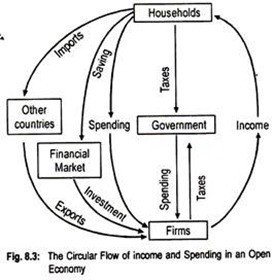
In other words, in an open economy, there occurs a trading relationship between nations. The circular flow model in a four-sector open economy has been shown in Fig. 8.3. Adding (X – M) in the above equation, we get

Y = C + I + G + (X – M)

The only difference in the circular flow of income between a closed economy and an open economy is that, in a four-sector economy, households purchase foreign-made goods and services (i.e., imports). Likewise, people of other countries purchase goods and services not produced domestically (i.e., exports).

Imports constitute leakage from the circular flow while exports constitute injection in the circular flow. For simplicity’s sake, we have not shown in the diagram that firms and governments also sell export goods and purchase import goods.

Note that (I + G + X) constitute injections into the circular flow of income while(S + T + M) constitute withdrawals or leakages from the circular flow of income. Injections increase national income and leakages decrease national income.

The national product or national income measures the overall economic performance of a nation. To measure the national product, we add up the value of all final goods and services produced in a country in a year. Thus, we focus on firms or sellers which receive payment for the production. This is the product method of calculating national income.

Leakages (withdrawals) from the circular flow

Not all income will flow from households to businesses directly. The circular flow shows that some part of household income will be:

• Put aside for future spending, i.e. savings (S) in banks accounts and other types of deposit
• Paid to the government in taxation (T) e.g. income tax and national insurance
• Spent on foreign-made goods and services, i.e. imports (M) which flow into the economy

Withdrawals are increases in savings, taxes or imports so reducing the circular flow of income and leading to a multiplied contraction of production (output)

Injections into the circular flow are additions to investment, government spending or exports so boosting the circular flow of income leading to a multiplied expansion of output.

• Capital spending by firms, i.e. investment expenditure (I) e.g. on new technology
• The government, i.e. government expenditure (G) e.g. on the NHS or defence
• Overseas consumers buying UK goods and service, i.e. UK export expenditure (X)

An economy is in equilibrium when the rate of injections = the rate of withdrawals from the circular flow.