Conditional Probability

Conditional probability refers to the probability of an event occurring, given that another event has already occurred. It quantifies the likelihood of one event under the condition that the related event is known.

The probability of the occurrence of an event A given that an event B has already occurred is called the conditional probability of A given B:

The same is explained in Figure 2.15 using the sample spaces related to the events A and B, assuming that there are few sample points common to these two events. Part 1 of the figure shows the total sample space related to the experiment as in the form of rectangle and the sample space related to the event A as a circle. Similarly part 2 of the figure shows the total sample space and the sample space related to event B. As explained earlier in conditional probability the total sample space is restrained to the sample space that is related to event B (which has already occurred). The same is shown in part 3 of Figure 2.15. Now the sample space for event A (B is the total sample space available) is nothing but the sample points related to event A and falling in the sample space. This is nothing but the intersection of the events A and B and is shown in part 3 of the figure as the hatched area.  

Figure 2.15: Representation of conditional probability using the Venn diagrams

For example, there are 100 trips per day between two places X and Y. Out of these 100 trips 50 are made by car, 25 are made by bus and the other 25 are by local train. Probabilities associated to these modes are 0.5, 0.25, and 0.25, respectively. In transportation engineering both the bus and the local train are considered as public transport so the event space associated to this is the summation of the event spaces associated to bus and local train. Probability of choosing public transportation is 0.5. Now if one is interested in finding the probability of choosing bus given public transportation is chosen the conditional probability is useful in finding that.

Addition and Multiplication Theorems

Addition Theorem on probability:

If A and B are any two events then the probability of happening of at least one of the events is defined as P(AUB) = P(A) + P(B)- P(A∩B).

Since events are nothing but sets,

From set theory, we have

n(AUB) = n(A) + n(B)- n(A∩B).

Dividing the above equation by n(S), (where S is the sample space)

n(AUB)/ n(S) = n(A)/ n(S) + n(B)/ n(S)- n(A∩B)/ n(S)

Then by the definition of probability,

P(AUB) = P(A) + P(B)- P(A∩B).

Example:

If the probability of solving a problem by two students George and James are 1/2 and 1/3 respectively then what is the probability of the problem to be solved.

Solution:

Let A and B be the probabilities of solving the problem by George and James respectively.

Then P(A)=1/2 and P(B)=1/3.

The problem will be solved if it is solved at least by one of them also.

So, we need to find P(AUB).

By addition theorem on probability, we have

P(AUB) = P(A) + P(B)- P(A∩B).

P(AUB) = 1/2 +.1/3 – 1/2 * 1/3 = 1/2 +1/3-1/6 = (3+2-1)/6 = 4/6 = 2/3

Note:

If A and B are any two mutually exclusive events then P(A∩B)=0.

Then P(AUB) = P(A)+P(B).

Multiplication theorem on probability:

If A and B are any two events  of a sample space such that P(A) ≠0 and P(B)≠0, then

P(A∩B) = P(A) * P(B|A) = P(B) *P(A|B).

Example:  If P(A) =  1/5  P(B|A) =  1/3  then what is P(A∩B)?

Solution: P(A∩B) = P(A) * P(B|A) = 1/5 * 1/3 = 1/15

INDEPENDENT EVENTS:

Two events A and B are said to be independent if there is no change in the happening of an event with the happening of the other event.

i.e. Two events A and B are said to be independent if

P(A|B) = P(A) where P(B)≠0.

P(B|A) = P(B) where P(A)≠0.

i.e. Two events A and B are said to be independent if

P(A∩B) = P(A) * P(B).

Example:

While laying the pack of cards, let A be the event of drawing a diamond and B be the event of drawing an ace.

Then P(A) =  13/52 = 1/4 and P(B) =  4/52=1/13

Now, A∩B = drawing a king card from hearts.

Then P(A∩B) =  1/52

Now, P(A/B) = P(A∩B)/P(B) = (1/52)/(1/13) = 1/4 = P(A).

So, A and B are independent.

[Here, P(A∩B) = =    = P(A) * P(B)]

Note:

(1)    If 3 events A,B and C are independent the

P(A∩B∩C) = P(A)*P(B)*P(C).

(2)    If A and B are any two events, then P(AUB) = 1-P(A’)P(B’).

Probability Meaning and Approaches of Probability Theory

In our day to day life the “probability” or “chance” is very commonly used term. Sometimes, we use to say “Probably it may rain tomorrow”, “Probably Mr. X may come for taking his class today”, “Probably you are right”. All these terms, possibility and probability convey the same meaning. But in statistics probability has certain special connotation unlike in Layman’s view.

The theory of probability has been developed in 17th century. It has got its origin from games, tossing coins, throwing a dice, drawing a card from a pack. In 1954 Antoine Gornband had taken an initiation and an interest for this area.

After him many authors in statistics had tried to remodel the idea given by the former. The “probability” has become one of the basic tools of statistics. Sometimes statistical analysis becomes paralyzed without the theorem of probability. Probability of a given event is defined as the expected frequency of occurrence of the event among events of a like sort.” (Garrett)

The probability theory provides a means of getting an idea of the likelihood of occurrence of different events resulting from a random experiment in terms of quantitative measures ranging between zero and one. The probability is zero for an impossible event and one for an event which is certain to occur.

Approaches of Probability Theory

  1. Classical Probability:

The classical approach to probability is one of the oldest and simplest school of thought. It has been originated in 18th century which explains probability concerning games of chances such as throwing coin, dice, drawing cards etc.

The definition of probability has been given by a French mathematician named “Laplace”. According to him probability is the ratio of the number of favourable cases among the number of equally likely cases.

Or in other words, the ratio suggested by classical approach is:

Pr. = Number of favourable cases/Number of equally likely cases

For example, if a coin is tossed, and if it is asked what is the probability of the occurrence of the head, then the number of the favourable case = 1, the number of the equally likely cases = 2.

Pr. of head = 1/2

Symbolically it can be expressed as:

P = Pr. (A) = a/n, q = Pr. (B) or (not A) = b/n

1 – a/n = b/n = (or) a + b = 1 and also p + q = 1

p = 1 – q, and q = 1 – p and if a + b = 1 then so also a/n + b/n = 1

In this approach the probability varies from 0 to 1. When probability is zero it denotes that it is impossible to occur.

If probability is 1 then there is certainty for occurrence, i.e. the event is bound to occur.

Example:

From a bag containing 20 black and 25 white balls, a ball is drawn randomly. What is the probability that it is black.

Pr. of a black ball = 20/45 = 4/9 = p, 25 Pr. of a white ball = 25/45 = 5/9 = q

p = 4/9 and q = 5/9 (p + q= 4/9 + 5/9= 1)

  1. Relative Frequency Theory of Probability:

This approach to probability is a protest against the classical approach. It indicates the fact that if n is increased upto the ∞, we can find out the probability of p or q.

Example:

If n is ∞, then Pr. of A= a/n = .5, Pr. of B = b/n = 5

If an event occurs a times out of n its relative frequency is a/n. When n becomes ∞, is called the limit of relative frequency.

Pr. (A) = limit a/n

where n → ∞

Pr. (B) = limit bl.t. here → ∞.

Axiomatic approach

An axiomatic approach is taken to define probability as a set function where the elements of the domain are the sets and the elements of range are real numbers. If event A is an element in the domain of this function, P(A) is the customary notation used to designate the corresponding element in the range.

Probability Function

A probability function p(A) is a function mapping the event space A of a random experiment into the interval [0,1] according to the following axioms;

Axiom 1. For any event A, 0 ≤ P(A) ≤ 1

Axiom 2. P(Ω) = 1

Axiom 3. If A and B are any two mutually exclusive events then,

                              P(A ∪ B)) = P(A) + P(B)

As given in the third axiom the addition property of the probability can be extended to any number of events as long as the events are mutually exclusive. If the events are not mutually exclusive then;

P(A ∪ B) = P(A) + P(B) – P(A∩B)

P(A∩B) is Φ if both the events are mutually exclusive.

If there are two types of objects among the objects of similar or other natures then the probability of one object i.e. Pr. of A = .5, then Pr. of B = .5

Lines of Regression; Co-efficient of regression

Regression Line is the line that best fits the data, such that the overall distance from the line to the points (variable values) plotted on a graph is the smallest. In other words, a line used to minimize the squared deviations of predictions is called as the regression line.

There are as many numbers of regression lines as variables. Suppose we take two variables, say X and Y, then there will be two regression lines:

  • Regression line of Y on X: This gives the most probable values of Y from the given values of X.
  • Regression line of X on Y: This gives the most probable values of X from the given values of Y.

The algebraic expression of these regression lines is called as Regression Equations. There will be two regression equations for the two regression lines.

The correlation between the variables depend on the distance between these two regression lines, such as the nearer the regression lines to each other the higher is the degree of correlation, and the farther the regression lines to each other the lesser is the degree of correlation.

The correlation is said to be either perfect positive or perfect negative when the two regression lines coincide, i.e. only one line exists. In case, the variables are independent; then the correlation will be zero, and the lines of regression will be at right angles, i.e. parallel to the X axis and Y axis.

The regression lines cut each other at the point of average of X and Y. This means, from the point where the lines intersect each other the perpendicular is drawn on the X axis we will get the mean value of X. Similarly, if the horizontal line is drawn on the Y axis we will get the mean value of Y.

Co-efficient of Regression

The Regression Coefficient is the constant ‘b’ in the regression equation that tells about the change in the value of dependent variable corresponding to the unit change in the independent variable.

If there are two regression equations, then there will be two regression coefficients:

  • Regression Coefficient of X on Y:

The regression coefficient of X on Y is represented by the symbol bxy that measures the change in X for the unit change in Y. Symbolically, it can be represented as:

The bxy can be obtained by using the following formula when the deviations are taken from the actual means of X and Y:When the deviations are obtained from the assumed mean, the following formula is used:

  • Regression Coefficient of Y on X:

The symbol byx is used that measures the change in Y corresponding to the unit change in X. Symbolically, it can be represented as:


In case, the deviations are taken from the actual means; the following formula is used:
The byx can be  calculated by using the following formula when the deviations are taken from the assumed means:

The Regression Coefficient is also called as a slope coefficient because it determines the slope of the line i.e. the change in the independent variable for the unit change in the independent variable

Difference between Correlation and Regression

Correlation and Regression

Correlation and regression are two important statistical tools used to study the relationship between variables. Both help managers analyze data and make informed business decisions. While correlation measures the degree and direction of relationship between variables, regression explains the cause-and-effect relationship and helps in prediction. Though closely related, their objectives and applications are different.

Correlation

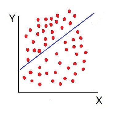
The term correlation is a combination of two words ‘Co’ (together) and relation (connection) between two quantities. Correlation is when, at the time of study of two variables, it is observed that a unit change in one variable is retaliated by an equivalent change in another variable, i.e. direct or indirect. Or else the variables are said to be uncorrelated when the movement in one variable does not amount to any movement in another variable in a specific direction. It is a statistical technique that represents the strength of the connection between pairs of variables.

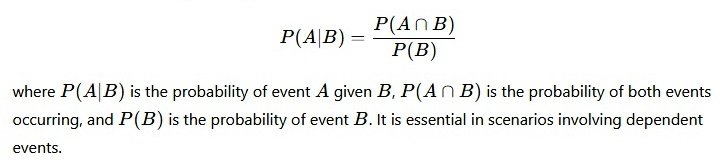
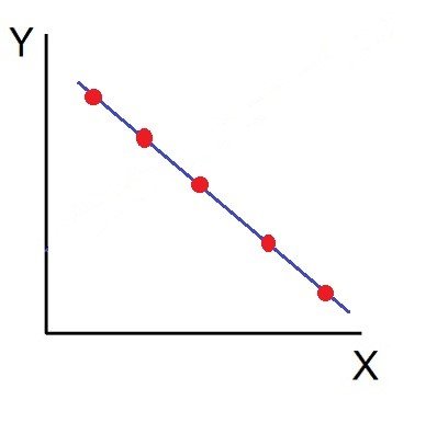
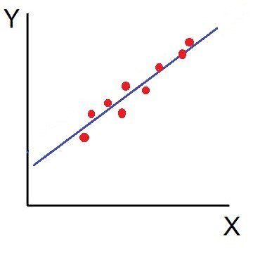
Correlation refers to a statistical measure that indicates the extent and direction of relationship between two variables. It shows whether variables move together or in opposite directions. Correlation is expressed numerically through the correlation coefficient (r), whose value lies between –1 and +1. A positive value indicates direct relationship, a negative value indicates inverse relationship, and zero indicates no relationship. Correlation does not indicate causation; it only measures association.

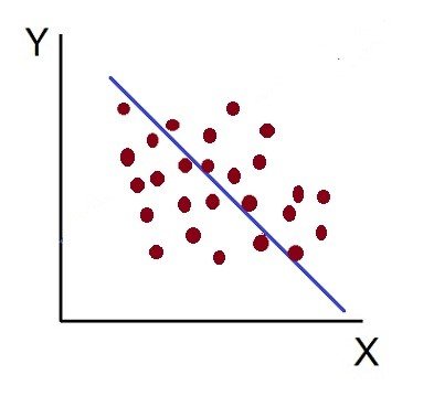
On the contrary, when the two variables move in different directions, in such a way that an increase in one variable will result in a decrease in another variable and vice versa, This situation is known as negative correlation. For instance: Price and demand of a product.

The measures of correlation are given as under:

  • Karl Pearson’s Product-moment correlation coefficient
  • Spearman’s rank correlation coefficient
  • Scatter diagram
  • Coefficient of concurrent deviations

Regression

Regression analysis is a statistical technique that establishes a functional or causal relationship between a dependent variable and one or more independent variables. It helps estimate or predict the value of one variable based on the known value of another. Regression provides a mathematical equation that explains how much change in the dependent variable is caused by changes in independent variables. It is widely used in forecasting and planning.

Differences Between Correlation and Regression

1. Meaning and Concept

Correlation and regression differ fundamentally in their basic meaning and conceptual approach. Correlation is a statistical measure that shows the degree and direction of relationship between two variables. It simply answers the question of whether variables are related and how strongly they move together. It does not explain why the relationship exists.

Regression, on the other hand, is a statistical technique that establishes a functional or causal relationship between variables. It explains how one variable (dependent) is affected by changes in another variable (independent). Regression goes beyond association and attempts to quantify the impact of one variable on another. Thus, while correlation is concerned with measuring association, regression focuses on explanation and prediction, making it more powerful for business decision-making.

2. Objective of Study

The objective of correlation is to determine whether a relationship exists between variables and to measure its strength and direction. It helps analysts understand patterns and tendencies in data. Correlation answers questions like: Are sales and advertising related? or Do income and consumption move together?

The objective of regression is to predict or estimate the value of one variable based on another. It is used when a business wants to forecast outcomes, such as predicting sales based on price or estimating costs based on output. Regression analysis provides a mathematical equation that can be used for planning, control, and forecasting. Hence, correlation is mainly descriptive in nature, while regression is both descriptive and predictive, making regression more suitable for managerial decision-making

3. Nature of Relationship

Correlation measures the degree of linear relationship between variables but does not indicate any cause-and-effect connection. Even if two variables are highly correlated, one may not necessarily cause changes in the other. For example, ice cream sales and electricity consumption may show correlation due to seasonal effects, not causation.

Regression, in contrast, assumes a cause-and-effect relationship between variables. It explains how changes in the independent variable bring about changes in the dependent variable. For instance, regression can estimate how much sales will increase due to a specific increase in advertising expenditure. Thus, correlation reflects association only, whereas regression attempts to establish dependence, which is crucial for business forecasting and strategic planning.

4. Treatment of Variables

In correlation, variables are treated symmetrically. There is no distinction between dependent and independent variables. The correlation between X and Y is the same as the correlation between Y and X. Both variables are given equal importance, and the analysis does not require identifying which variable influences the other.

In regression, variables are treated asymmetrically. One variable is clearly identified as the dependent variable, and the other(s) as independent variables. The entire analysis is based on explaining or predicting the dependent variable. For example, sales may depend on price and advertising. This clear distinction is essential for regression analysis, making it more suitable for practical business applications where cause-and-effect relationships are required.

5. Numerical Measure and Output

Correlation is expressed using a single numerical value, called the correlation coefficient (r). This value ranges from –1 to +1 and indicates only the strength and direction of relationship. A single figure summarizes the entire relationship, which makes correlation easy to compute and interpret but limited in analytical depth.

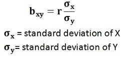
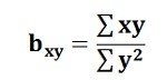
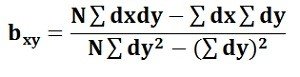
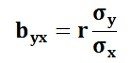
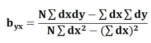
Regression produces regression equations, such as Y = a + bX, where coefficients show the magnitude of change in the dependent variable due to a unit change in the independent variable. These equations provide detailed quantitative insights and allow prediction. Therefore, while correlation provides a summary measure, regression offers a complete analytical model useful for forecasting and decision-making.

6. Symmetry and Direction

Correlation is symmetric in nature, meaning that correlation between X and Y is exactly the same as correlation between Y and X. There is no concept of direction of dependence in correlation analysis. This symmetry limits its usefulness in predictive analysis.

Regression is not symmetric. Regression of Y on X is different from regression of X on Y. Each regression equation serves a specific purpose depending on which variable is treated as dependent. This directional nature makes regression a powerful analytical tool. It helps managers decide which variable should be predicted and which variables should be used as predictors, making regression more practical for real-world business problems.

7. Use in Prediction and Forecasting

Correlation is not suitable for prediction. Although it indicates the existence of a relationship, it does not provide a mechanism to estimate future values. A high correlation does not necessarily mean accurate forecasting is possible.

Regression is specifically designed for prediction and forecasting. Using regression equations, businesses can estimate future sales, costs, profits, or demand based on known values of independent variables. This makes regression extremely valuable for planning, budgeting, and policy formulation. Thus, correlation is primarily exploratory, while regression is predictive and decision-oriented.

8. Practical Application in Business

Correlation is mainly used for preliminary analysis. It helps identify whether variables are related and whether further analysis is worthwhile. For example, before performing regression, managers often check correlation to see if a relationship exists.

Regression has direct practical applications in business, including sales forecasting, demand estimation, cost control, pricing decisions, and investment analysis. It provides a scientific basis for managerial decisions. Hence, correlation serves as a starting point in analysis, while regression forms the foundation of advanced quantitative decision-making in business.

Key Differences Between Correlation and Regression

Aspect Correlation Regression
Meaning Correlation measures the degree and direction of relationship between two variables. Regression measures the functional and causal relationship between variables.
Nature It shows association only. It shows cause-and-effect relationship.
Objective To determine whether variables are related and how strongly. To predict or estimate the value of one variable from another.
Type of Relationship Indicates linear association only. Explains dependence of one variable on another.
Variables Does not distinguish between dependent and independent variables. Clearly distinguishes dependent and independent variables.
Direction of Influence No direction of influence is implied. Direction of influence is clearly defined.
Numerical Measure Expressed through a single value called correlation coefficient (r). Expressed through regression equations.
Range of Values Lies between –1 and +1. No fixed range for regression coefficients.
Symmetry Symmetric in nature (X with Y = Y with X). Asymmetric (Regression of Y on X ≠ X on Y).
Use in Prediction Not suitable for prediction. Specifically used for forecasting and prediction.
Number of Equations Only one coefficient is calculated. Two regression equations can be formed.
Dependency Assumption No assumption of dependency. Assumes dependency of one variable on another.
Effect of Change in Units Correlation coefficient is unit-free. Regression coefficients depend on measurement units.
Business Application Used mainly for preliminary analysis. Widely used for decision-making and planning.
Analytical Depth Provides limited analytical insight. Provides detailed quantitative analysis.

Rank correlation; coefficient of determination

Rank Correlation

Sometimes there doesn’t exist a marked linear relationship between two random variables but a monotonic relation (if one increases, the other also increases or instead, decreases) is clearly noticed. A Pearson’s Correlation Coefficient evaluation, in this case, would give us the strength and direction of the linear association only between the variables of interest. Herein comes the advantage of the Spearman Rank Correlation methods, which will instead, give us the strength and direction of the monotonic relation between the connected variables. This can be a good starting point for further evaluation.

The Spearman Rank Order Correlation Coefficient

The Spearman’s Correlation Coefficient, represented by ρ or by rR, is a nonparametric measure of the strength and direction of the association that exists between two ranked variables. It determines the degree to which a relationship is monotonic, i.e., whether there is a monotonic component of the association between two continuous or ordered variables.

Monotonicity is “less restrictive” than that of a linear relationship. Although monotonicity is not actually a requirement of Spearman’s correlation, it will not be meaningful to pursue Spearman’s correlation to determine the strength and direction of a monotonic relationship if we already know the relationship between the two variables is not monotonic.

On the other hand if, for example, the relationship appears linear (assessed via scatterplot) one would run a Pearson’s correlation because this will measure the strength and direction of any linear relationship.

Spearman Ranking of the Data

We must rank the data under consideration before proceeding with the Spearman’s Rank Correlation evaluation. This is necessary because we need to compare whether on increasing one variable, the other follows a monotonic relation (increases or decreases regularly) with respect to it or not.

Thus, at every level, we need to compare the values of the two variables. The method of ranking assigns such ‘levels’ to each value in the dataset so that we can easily compare it.

  • Assign number 1 to n (the number of data points) corresponding to the variable values in the order highest to lowest.
  • In the case of two or more values being identical, assign to them the arithmetic mean of the ranks that they would have otherwise occupied.

The Formula for Spearman Rank Correlation

where is the number of data points of the two variables and di is the difference in the ranks of the ith element of each random variable considered. The Spearman correlation coefficient, ρ, can take values from +1 to -1.

  • A ρ of +1 indicates a perfect association of ranks
  • A ρ of zero indicates no association between ranks and
  • ρ of -1 indicates a perfect negative association of ranks.
    The closer ρ is to zero, the weaker the association between the ranks.

Coefficient of Determination

The Coefficient of determination is the square of the coefficient of correlation r2 which is calculated to interpret the value of the correlation. It is useful because it explains the level of variance in the dependent variable caused or explained by its relationship with the independent variable.

The coefficient of determination explains the proportion of the explained variation or the relative reduction in variance corresponding to the regression equation rather than about the mean of the dependent variable. For example, if the value of r = 0.8, then r2 will be 0.64, which means that 64% of the variation in the dependent variable is explained by the independent variable while 36% remains unexplained.

Thus, the coefficient of determination is the ratio of explained variance to the total variance that tells about the strength of linear association between the variables, say X and Y. The value of r2 lies between 0 and 1 and observes the following relationship with ‘r’.

  • With the decrease in the value of ‘r’ from its maximum value of 1, the ‘r2’ also decreases much more rapidly.
  • The value of ‘r’ will always be greater than ‘r2’ unless the r2=0 or 1.

The coefficient of determination also explains that how well the regression line fits the statistical data. The closer the regression line to the points plotted on a scatter diagram, the more likely it explains all the variation and the farther the line from the points the lesser is the ability to explain the variance.

Properties of Correlation co-efficient

The following are the main properties of correlation.

  1. Coefficient of Correlation lies between -1 and +1:

The coefficient of correlation cannot take value less than -1 or more than one +1. Symbolically,

-1<=r<= + 1 or | r | <1.

  1. Coefficients of Correlation are independent of Change of Origin:

This property reveals that if we subtract any constant from all the values of X and Y, it will not affect the coefficient of correlation.

  1. Coefficients of Correlation possess the property of symmetry:

The degree of relationship between two variables is symmetric as shown below:

  1. Coefficient of Correlation is independent of Change of Scale:

This property reveals that if we divide or multiply all the values of X and Y, it will not affect the coefficient of correlation.

  1. Co-efficient of correlation measures only linear correlation between X and Y.
  2. If two variables X and Y are independent, coefficient of correlation between them will be zero.

Karl Pearson’s Coefficient of Correlation is widely used mathematical method wherein the numerical expression is used to calculate the degree and direction of the relationship between linear related variables.

Pearson’s method, popularly known as a Pearsonian Coefficient of Correlation, is the most extensively used quantitative methods in practice. The coefficient of correlation is denoted by “r”.

If the relationship between two variables X and Y is to be ascertained, then the following formula is used:

Properties of Coefficient of Correlation

  • The value of the coefficient of correlation (r) always lies between±1. Such as:
    r=+1, perfect positive correlation
    r=-1, perfect negative correlation
    r=0, no correlation
  • The coefficient of correlation is independent of the origin and scale.By origin, it means subtracting any non-zero constant from the given value of X and Y the vale of “r” remains unchanged. By scale it means, there is no effect on the value of “r” if the value of X and Y is divided or multiplied by any constant.
  • The coefficient of correlation is a geometric mean of two regression coefficient.Symbolically it is represented as:
  • The coefficient of correlation is “zero”when the variables X and Y are independent. But, however, the converse is not true.

Assumptions of Karl Pearson’s Coefficient of Correlation

  1. The relationship between the variables is “Linear”,which means when the two variables are plotted, a straight line is formed by the points plotted.
  2. There are a large number of independent causes that affect the variables under study so as to form a Normal Distribution. Such as, variables like price, demand, supply, etc. are affected by such factors that the normal distribution is formed.
  3. The variables are independent of each other.

Note: The coefficient of correlation measures not only the magnitude of correlation but also tells the direction. Such as, r = -0.67, which shows correlation is negative because the sign is “-“and the magnitude is 0.67.

Scatter Diagram

Scatter Diagram Method is the simplest method to study the correlation between two variables wherein the values for each pair of a variable is plotted on a graph in the form of dots thereby obtaining as many points as the number of observations. Then by looking at the scatter of several points, the degree of correlation is ascertained.

The degree to which the variables are related to each other depends on the manner in which the points are scattered over the chart. The more the points plotted are scattered over the chart, the lesser is the degree of correlation between the variables. The more the points plotted are closer to the line, the higher is the degree of correlation. The degree of correlation is denoted by “r”.

The following types of scatter diagrams tell about the degree of correlation between variable X and variable Y.

  1. Perfect Positive Correlation (r = +1):

The correlation is said to be perfectly positive when all the points lie on the straight line rising from the lower left-hand corner to the upper right-hand corner.

2. Perfect Negative Correlation (r = -1):

When all the points lie on a straight line falling from the upper left-hand corner to the lower right-hand corner, the variables are said to be negatively correlated.

3. High Degree of +Ve Correlation (r = + High):

The degree of correlation is high when the points plotted fall under the narrow band and is said to be positive when these show the rising tendency from the lower left-hand corner to the upper right-hand corner.

4. High Degree of –Ve Correlation (r = – High):

The degree of negative correlation is high when the point plotted fall in the narrow band and show the declining tendency from the upper left-hand corner to the lower right-hand corner.

5. Low degree of +Ve Correlation (r = + Low):

The correlation between the variables is said to be low but positive when the points are highly scattered over the graph and show a rising tendency from the lower left-hand corner to the upper right-hand corner.

6. Low Degree of –Ve Correlation (r = + Low):

The degree of correlation is low and negative when the points are scattered over the graph and the show the falling tendency from the upper left-hand corner to the lower right-hand corner.

7. No Correlation (r = 0):

The variable is said to be unrelated when the points are haphazardly scattered over the graph and do not show any specific pattern. Here the correlation is absent and hence r = 0.

Thus, the scatter diagram method is the simplest device to study the degree of relationship between the variables by plotting the dots for each pair of variable values given. The chart on which the dots are plotted is also called as a Dotogram.

Methods of Studying Correlation

The Correlation is a statistical tool used to measure the relationship between two or more variables, i.e. the degree to which the variables are associated with each other, such that the change in one is accompanied by the change in another.

The correlation is said to be linear when the change in the amount of one variable tends to bear a constant ratio to the amount of change in another variable. Whereas, the non-linear or curvilinear correlation is when the ratio of the amount of change in one variable to the amount of change in another variable is not constant.

These figures clearly show the difference between the linear and non-linear correlation. To determine the linearity and non-linearity among the variables and the extent to which these are correlated, following are the important methods used to ascertain these:

  1. Scatter Diagram Method
  2. Karl Pearson’s Coefficient of Correlation
  3. Spearman’s Rank Correlation Coefficient; and
  4. Methods of Least Squares

Among these, the first method, i.e. scatter diagram method is based on the study of graphs while the rest is mathematical methods that use formulae to calculate the degree of correlation between the variables.  The researcher may apply either of these methods on the basis of the nature of variables being considered in ascertaining the association between them.

Positive and Negative Correlation

Correlation can be defined as a statistical tool that defines the relationship between two variables. For, eg: correlation may be used to define the relationship between the price of a good and its quantity demanded. It explains how two variables are related but do not explain any cause-effect relation. It only gives an understanding as to the direction and intensity of relation between two variables. Correlation can be of two types:

A) Positive Correlation

A correlation in the same direction is called a positive correlation. If one variable increases the other also increases and when one variable decreases the other also decreases. For example, the length of an iron bar will increase as the temperature increases.

Two variables are positively correlated when they move together in the same direction. In economics, quantity supplied increases as the price increases. This is because sellers find it profitable to sell when the prices are high, so they will sell more. Thus, we can call price and quantity supplied to be positively correlated. This is also called the law of supply.

B) Negative Correlation

Correlation in the opposite direction is called a negative correlation. Here if one variable increases the other decreases and vice versa. For example, the volume of gas will decrease as the pressure increases, or the demand for a particular commodity increases as the price of such commodity decreases.

Two variables are negatively correlated if they move in opposite directions. For instance, as the price of increases, the quantity demanded declines as the good becomes more expensive relative to when the price had not increased. Thus, we can say that price and quantity demanded are negatively correlated. Note that this is the famous law of demand.

C) No Correlation or Zero Correlation

If there is no relationship between the two variables such that the value of one variable changes and the other variable remains constant, it is called no or zero correlation.

Simple, Partial and Multiple Correlation: Whether the correlation is simple, partial or multiple depends on the number of variables studied. The correlation is said to be simple when only two variables are studied. The correlation is either multiple or partial when three or more variables are studied. The correlation is said to be Multiple when three variables are studied simultaneously. Such as, if we want to study the relationship between the yield of wheat per acre and the amount of fertilizers and rainfall used, then it is a problem of multiple correlations.

Whereas, in the case of a partial correlation we study more than two variables, but consider only two among them that would be influencing each other such that the effect of the other influencing variable is kept constant. Such as, in the above example, if we study the relationship between the yield and fertilizers used during the periods when certain average temperature existed, then it is a problem of partial correlation.

error: Content is protected !!