Tag: Correlation Analysis

In statistical hypothesis testing, a type I error is the incorrect rejection of a true null hypothesis (also known as a “false positive” finding), while a type II error is incorrectly retaining a false null hypothesis (also known as a “false negative” finding). More simply stated, a type I error is to falsely infer the existence of something that is not there, while a type II error is to falsely infer the absence of something that is.

A type I error (or error of the first kind) is the incorrect rejection of a true null hypothesis. Usually a type I error leads one to conclude that a supposed effect or relationship exists when in fact it doesn’t. Examples of type I errors include a test that shows a patient to have a disease when in fact the patient does not have the disease, a fire alarm going on indicating a fire when in fact there is no fire, or an experiment indicating that a medical treatment should cure a disease when in fact it does not.

A type II error (or error of the second kind) is the failure to reject a false null hypothesis. Examples of type II errors would be a blood test failing to detect the disease it was designed to detect, in a patient who really has the disease; a fire breaking out and the fire alarm does not ring; or a clinical trial of a medical treatment failing to show that the treatment works when really it does.

When comparing two means, concluding the means were different when in reality they were not different would be a Type I error; concluding the means were not different when in reality they were different would be a Type II error. Various extensions have been suggested as “Type III errors”, though none have wide use.

All statistical hypothesis tests have a probability of making type I and type II errors. For example, all blood tests for a disease will falsely detect the disease in some proportion of people who don’t have it, and will fail to detect the disease in some proportion of people who do have it. A test’s probability of making a type I error is denoted by α. A test’s probability of making a type II error is denoted by β. These error rates are traded off against each other: for any given sample set, the effort to reduce one type of error generally results in increasing the other type of error. For a given test, the only way to reduce both error rates is to increase the sample size, and this may not be feasible.

Type I error

A type I error occurs when the null hypothesis (H0) is true, but is rejected. It is asserting something that is absent, a false hit. A type I error may be likened to a so-called false positive (a result that indicates that a given condition is present when it actually is not present).

In terms of folk tales, an investigator may see the wolf when there is none (“raising a false alarm”). Where the null hypothesis, H0, is: no wolf.

The type I error rate or significance level is the probability of rejecting the null hypothesis given that it is true. It is denoted by the Greek letter α (alpha) and is also called the alpha level. Often, the significance level is set to 0.05 (5%), implying that it is acceptable to have a 5% probability of incorrectly rejecting the null hypothesis.

Type II error

A type II error occurs when the null hypothesis is false, but erroneously fails to be rejected. It is failing to assert what is present, a miss. A type II error may be compared with a so-called false negative (where an actual ‘hit’ was disregarded by the test and seen as a ‘miss’) in a test checking for a single condition with a definitive result of true or false. A Type II error is committed when we fail to believe a true alternative hypothesis.

In terms of folk tales, an investigator may fail to see the wolf when it is present (“failing to raise an alarm”). Again, H0: no wolf.

The rate of the type II error is denoted by the Greek letter β (beta) and related to the power of a test (which equals 1−β).

Aspect	Type-I Error (False Positive)	Type-II Error (False Negative)
Definition	Rejecting a true null hypothesis.	Failing to reject a false null hypothesis.
Symbol	Denoted as α (significance level).	Denoted as β.
Outcome	Concluding that there is an effect when there isn’t.	Concluding that there is no effect when there is.
Risk	Risk of concluding a false discovery.	Risk of missing a true effect.
Example	Concluding a new drug is effective when it isn’t.	Concluding a drug is ineffective when it is.
Critical Value	Occurs when the test statistic exceeds the critical value.	Occurs when the test statistic does not exceed the critical value.
Relation to Power	As α decreases, the probability of Type-I error decreases.	As β increases, the probability of Type-II error increases.
Control	Controlled by choosing the significance level (α).	Controlled by increasing the sample size or improving the test’s power.

T-test

A t-test is a statistical test used to determine if there is a significant difference between the means of two independent groups or samples. It allows researchers to assess whether the observed difference in sample means is likely due to a real difference in population means or just due to random chance.

The t-test is based on the t-distribution, which is a probability distribution that takes into account the sample size and the variability within the samples. The shape of the t-distribution is similar to the normal distribution, but it has fatter tails, which accounts for the greater uncertainty associated with smaller sample sizes.

Assumptions of T-test

The t-test relies on several assumptions to ensure the validity of its results. It is important to understand and meet these assumptions when performing a t-test.

• Independence:

The observations within each sample should be independent of each other. In other words, the values in one sample should not be influenced by or dependent on the values in the other sample.

• Normality:

The populations from which the samples are drawn should follow a normal distribution. While the t-test is fairly robust to departures from normality, it is more accurate when the data approximate a normal distribution. However, if the sample sizes are large enough (typically greater than 30), the t-test can be applied even if the data are not perfectly normally distributed due to the Central Limit Theorem.

• Homogeneity of variances:

The variances of the populations from which the samples are drawn should be approximately equal. This assumption is also referred to as homoscedasticity. Violations of this assumption can affect the accuracy of the t-test results. In cases where the variances are unequal, there are modified versions of the t-test that can be used, such as the Welch’s t-test.

Types of T-test

There are three main types of t-tests:

• Independent samples t-test:

This type of t-test is used when you want to compare the means of two independent groups or samples. For example, you might compare the mean test scores of students who received a particular teaching method (Group A) with the mean test scores of students who received a different teaching method (Group B). The test determines if the observed difference in means is statistically significant.

• Paired samples t-test:

This t-test is used when you want to compare the means of two related or paired samples. For instance, you might measure the blood pressure of individuals before and after a treatment and want to determine if there is a significant difference in blood pressure levels. The paired samples t-test accounts for the correlation between the two measurements within each pair.

• One-sample t-test:

This t-test is used when you want to compare the mean of a single sample to a known or hypothesized population mean. It allows you to assess if the sample mean is significantly different from the population mean. For example, you might want to determine if the average weight of a sample of individuals is significantly different from a specified value.

The t-test also involves specifying a level of significance (e.g., 0.05) to determine the threshold for considering a result statistically significant. If the calculated t-value falls beyond the critical value for the chosen significance level, it suggests a significant difference between the means.

Z-test

A z-test is a statistical test used to determine if there is a significant difference between a sample mean and a known population mean. It allows researchers to assess whether the observed difference in sample mean is statistically significant.

The z-test is based on the standard normal distribution, also known as the z-distribution. Unlike the t-distribution used in the t-test, the z-distribution is a well-defined probability distribution with known properties.

The z-test is typically used when the sample size is large (typically greater than 30) and either the population standard deviation is known or the sample standard deviation can be a good estimate of the population standard deviation.

Steps Involved in Conducting a Z-test

• Formulate hypotheses:

Start by stating the null hypothesis (H0) and alternative hypothesis (Ha) about the population mean. The null hypothesis typically assumes that there is no significant difference between the sample mean and the population mean.

• Calculate the test statistic:

The test statistic for a z-test is calculated as (sample mean – population mean) / (population standard deviation / sqrt(sample size)). This represents how many standard deviations the sample mean is away from the population mean.

• Determine the critical value:

The critical value is a threshold based on the chosen level of significance (e.g., 0.05) that determines whether the observed difference is statistically significant. The critical value is obtained from the z-distribution.

• Compare the test statistic with the critical value:

If the absolute value of the test statistic exceeds the critical value, it suggests a statistically significant difference between the sample mean and the population mean. In this case, the null hypothesis is rejected in favor of the alternative hypothesis.

• Calculate the p-value (optional):

The p-value represents the probability of obtaining a test statistic as extreme as, or more extreme than, the observed value, assuming the null hypothesis is true. If the p-value is smaller than the chosen level of significance, it indicates a statistically significant difference.

Assumptions of Z-test

• Random sample:

The sample should be randomly selected from the population of interest. This means that each member of the population has an equal chance of being included in the sample, ensuring representativeness.

• Independence:

The observations within the sample should be independent of each other. Each data point should not be influenced by or dependent on any other data point in the sample.

• Normal distribution or large sample size:

The z-test assumes that the population from which the sample is drawn follows a normal distribution. Alternatively, the sample size should be large enough (typically greater than 30) for the central limit theorem to apply. The central limit theorem states that the distribution of the sample mean approaches a normal distribution as the sample size increases, regardless of the shape of the population distribution.

• Known population standard deviation:

The z-test assumes that the population standard deviation (or variance) is known. This assumption is necessary for calculating the z-score, which is the test statistic used in the z-test.

Key differences between T-test and Z-test

Feature	T-Test	Z-Test
Purpose	Compare means of two independent or related samples	Compare mean of a sample to a known population mean
Distribution	T-Distribution	Standard Normal Distribution (Z-Distribution)
Sample Size	Small (typically < 30)	Large (typically > 30)
Population SD	Unknown or estimated from the sample	Known or assumed
Test Statistic	(Sample mean – Population mean) / (Standard error)	(Sample mean – Population mean) / (Population SD)
Assumption	Normality of populations, Independence	Normality (or large sample size), Independence
Variances	Assumes potentially unequal variances	Assumes equal variances (homoscedasticity)
Degrees of Freedom	(n1 + n2 – 2) for independent samples t-test	n – 1 for one-sample t-test, (n1 + n2 – 2) for others
Critical Values	Vary based on degrees of freedom and level of significance.	Fixed critical values based on level of significance
Use Cases	Comparing means of two groups, before-after analysis	Comparing a sample mean to a known population mean

Hypothesis testing is a systematic method used in statistics to determine whether there is enough evidence in a sample to infer a conclusion about a population.

1. Formulate the Hypotheses

The first step is to define the two hypotheses:

• Null Hypothesis (H_0​): Represents the assumption of no effect, relationship, or difference. It acts as the default statement to be tested.

  Example: “The new drug has no effect on blood pressure.”

• Alternative Hypothesis (H_1​): Represents what the researcher seeks to prove, suggesting an effect, relationship, or difference.

  Example: “The new drug significantly lowers blood pressure.”

2. Choose the Significance Level (α)

The significance level determines the threshold for rejecting the null hypothesis. Common choices include $\alpha =0.05$ (5%) or if $\alpha =0.01$ (1%). This value indicates the probability of rejecting H_0​ when it is true (Type I error).

3. Select the Appropriate Test

Choose a statistical test based on:

• The type of data (e.g., categorical, continuous).
• The sample size.
• The assumptions about the data distribution (e.g., normal distribution).

  Examples include t-tests, z-tests, chi-square tests, and ANOVA.

4. Collect and Summarize Data

Gather the sample data, ensuring it is representative of the population. Calculate the sample statistic (e.g., mean, proportion) relevant to the hypothesis being tested.

5. Compute the Test Statistic

Using the sample data, compute the test statistic (e.g., t-value, z-value) based on the chosen test. This statistic helps determine how far the sample data deviates from what is expected under H_0​.

6. Determine the P-Value

The p-value is the probability of observing the sample results (or more extreme) if H0H_0H0​ is true.

• If p-value ≤ $\alpha$: Reject H_0​ in favor of H_1​.
• If p-value > $\alpha$: Fail to reject H_0​.

7. Draw a Conclusion

Based on the p-value and test statistic, decide whether to reject or fail to reject H0H_0H0​.

• Reject H_0​: There is sufficient evidence to support H_1​.
• Fail to Reject H_0​: There is insufficient evidence to support H_1​.

8. Report the Results

Clearly communicate the findings, including the hypotheses, significance level, test statistic, p-value, and conclusion. This ensures transparency and allows others to validate the results.

Hypothesis Testing is a statistical method used to make decisions or draw conclusions about a population based on sample data. It involves formulating two opposing hypotheses: the null hypothesis (H₀), which assumes no effect or relationship, and the alternative hypothesis (H₁), which suggests a significant effect or relationship. The process tests whether the sample data provides enough evidence to reject H₀​ in favor of H₁​. Using a significance level (α), the test determines the probability of observing the sample data if H₀​ is true. Common methods include t-tests, z-tests, and chi-square tests.

Characteristics of Hypothesis:

• Testability

A good hypothesis must be testable through empirical observation or experimentation. This means it should make clear, measurable predictions that can be verified or disproven using data. A testable hypothesis avoids vague language and includes variables that can be quantified or observed in real-world situations. For instance, “Customer satisfaction improves sales” is testable if satisfaction and sales are properly defined and measured. Testability ensures that the hypothesis can undergo scientific scrutiny, allowing for validation or rejection based on evidence. Without testability, a hypothesis remains theoretical and cannot contribute meaningfully to research or decision-making.

• Falsifiability

A hypothesis must be falsifiable, meaning it can be proven wrong through evidence. This characteristic is essential for scientific inquiry, as it allows researchers to critically examine the hypothesis by attempting to disprove it. If a hypothesis cannot be refuted under any condition, it lacks scientific value. For example, “All swans are white” is falsifiable because the discovery of a single black swan disproves it. Falsifiability encourages objectivity and rigor, making it possible to separate valid hypotheses from those based on assumptions or beliefs. It keeps research grounded in observable facts rather than subjective interpretations.

• Clarity and Precision

A hypothesis must be clearly and precisely stated to avoid confusion and misinterpretation. It should define the variables involved and express the relationship between them in specific terms. Ambiguity or vague language can lead to inconsistent understanding and flawed research design. For example, “Social media affects youth” is unclear, while “Daily use of Instagram negatively affects academic performance among college students” is precise. Clarity ensures that all stakeholders—researchers, participants, and readers—understand exactly what is being studied, making it easier to develop valid methodologies and analyze results accurately.

• Specificity

Specificity ensures that the hypothesis focuses on a particular aspect or relationship, limiting the scope to manageable and researchable elements. A specific hypothesis includes well-defined variables, the direction of the expected relationship, and often the population or context. For instance, “Increased screen time reduces sleep quality among teenagers” is more specific than “Technology affects health.” Specific hypotheses help in selecting the right research design, sampling method, and data collection tools. They also allow for more accurate testing and interpretation of results. Being specific makes the hypothesis more useful and applicable in addressing the research problem effectively.

• Relevance

A hypothesis must be relevant to the research problem, objectives, and field of study. It should address a significant question or gap in knowledge that, when tested, contributes to theory or practice. Irrelevant hypotheses waste resources and divert attention from meaningful inquiry. For example, in a study on employee retention, a relevant hypothesis could be “Flexible work hours increase employee retention in the IT sector.” Relevance ensures that the findings from the research will provide useful insights or solutions. It aligns the hypothesis with real-world needs, making the research more impactful and valuable.

• Consistency with Existing Knowledge

A well-formulated hypothesis should align with existing theories, principles, or findings unless it intentionally seeks to challenge them. Consistency with established knowledge ensures that the hypothesis is grounded in reality and builds on previous research. For example, a hypothesis about the relationship between motivation and performance should be compatible with known motivational theories like Maslow’s or Herzberg’s. However, even if challenging established ideas, the hypothesis should do so logically and not contradict basic facts. This characteristic enhances the hypothesis’s credibility and acceptance within the academic or scientific community.

Formulation of Hypothesis Testing:

The formulation of hypothesis testing involves defining and structuring the hypotheses to analyze a research question or problem systematically. This process provides the foundation for statistical inference and ensures clarity in decision-making.

1. Define the Research Problem

• Clearly identify the problem or question to be addressed.
• Ensure the problem is specific, measurable, and achievable using statistical methods.

2. Establish Null and Alternative Hypotheses

• Null Hypothesis (H_0​): Represents the default assumption that there is no effect, relationship, or difference in the population.Example: “There is no difference in the average test scores of two groups.”
• Alternative Hypothesis (H_1​): Contradicts the null hypothesis and suggests a significant effect, relationship, or difference.Example: “The average test score of one group is higher than the other.”

3. Select the Type of Test

• Determine whether the test is one-tailed (specific direction) or two-tailed (both directions).
  • One-tailed test: Tests for an effect in a specific direction (e.g., greater than or less than).
  • Two-tailed test: Tests for an effect in either direction (e.g., not equal to).

4. Choose the Level of Significance (α)

The significance level represents the probability of rejecting the null hypothesis when it is true. Common values are $\alpha =0.05$ (5%) or $\alpha =0.01$ (1%).

5. Identify the Appropriate Test Statistic

Choose a test statistic based on data type and distribution, such as t-test, z-test, chi-square, or F-test.

6. Collect and Analyze Data

• Gather a representative sample and compute the test statistic using the collected data.
• Calculate the p-value, which indicates the probability of observing the sample data if the null hypothesis is true.

7. Make a Decision

• Reject H_0​ if the p-value is less than α, supporting H_1​.
• Fail to reject H_0​ if the p-value is greater than α, indicating insufficient evidence against H_0​.

Types of Hypothesis Testing:

Hypothesis testing methods are categorized based on the nature of the data and the research objective.

1. Parametric Tests

Parametric tests assume that the data follows a specific distribution, usually normal. These tests are more powerful when assumptions about the data are met. Common parametric tests include:

• t-Test: Compares the means of two groups (independent or paired samples).
• z-Test: Used for large sample sizes to compare means or proportions.
• ANOVA (Analysis of Variance): Compares means across three or more groups.
• F-Test: Compares variances between two populations.

2. Non-Parametric Tests

Non-parametric tests do not assume a specific data distribution, making them suitable for non-normal or ordinal data. Examples include:

• Chi-Square Test: Tests the independence or goodness-of-fit for categorical data.
• Mann-Whitney U Test: Compares medians between two independent groups.
• Kruskal-Wallis Test: Compares medians across three or more groups.
• Wilcoxon Signed-Rank Test: Compares paired or matched samples.

3. One-Tailed and Two-Tailed Tests

• One-Tailed Test: Tests the effect in one direction (e.g., greater or less than).
• Two-Tailed Test: Tests the effect in both directions, identifying whether it is significantly different without specifying the direction.

4. Null and Alternative Hypothesis Testing

• Null Hypothesis (H₀​): Assumes no effect or relationship.
• Alternative Hypothesis (H₁): Suggests a significant effect or relationship.

5. Tests for Correlation and Regression

• Pearson Correlation Test: Evaluates the linear relationship between two variables.
• Regression Analysis: Tests the dependency of one variable on another.

Correlation is a statistical concept that measures the degree of relationship between two or more variables. The main idea is to understand how one variable changes when another variable changes. For example, in business, understanding the relationship between advertising expenditure and sales revenue can help managers make informed decisions. Correlation focuses on association, not causation. This means that even if two variables move together, it does not imply that one causes the other; they may simply be related.

Meaning of Correlation

Correlation refers to a statistical measure that expresses the extent to which two variables are related. It is used to study the interdependence between variables. In a business context, correlation helps in analyzing patterns, forecasting trends, and making decisions based on observed relationships.

For instance:

• If sales increase with higher advertising expenditure, there is a positive correlation.

• If employee absenteeism increases while productivity decreases, there is a negative correlation.

Definitions of Correlation

• Karl Pearson (1896) – “Correlation is the degree to which one variable is linearly related to another variable.”

• Gosset (Student) – “Correlation is a statistical measure that shows the tendency of variables to vary together.”

• Croxton and Cowden – “Correlation is the degree of correspondence between two or more variables. It measures the extent to which changes in one variable are associated with changes in another.”

Significance of Correlation

• Identifies Relationships Between Variables

Correlation helps identify whether and how two variables are related. For instance, it can reveal if there is a relationship between factors like advertising spend and sales revenue. This insight helps businesses and researchers understand the dynamics at play, providing a foundation for further investigation.

• Predictive Power

Once a correlation between two variables is established, it can be used to predict the behavior of one variable based on the other. For example, if a strong positive correlation is found between temperature and ice cream sales, higher temperatures can predict increased sales. This predictive ability is especially valuable in decision-making processes in business, economics, and health.

• Guides Decision-Making

In business and economics, understanding correlations enables better decision-making. For example, a company can analyze the correlation between marketing activities and customer acquisition, allowing for better resource allocation and strategy formulation. Similarly, policymakers can examine correlations between economic indicators (e.g., unemployment rates and inflation) to make informed policy choices.

• Quantifies the Strength of Relationships

The correlation coefficient quantifies the strength of the relationship between variables. A higher correlation coefficient (close to +1 or -1) signifies a stronger relationship, while a coefficient closer to 0 indicates a weak relationship. This quantification helps in understanding how closely variables move together, which is crucial in areas like finance or research.

• Helps in Risk Management

In finance, correlation is used to assess the relationship between different investment assets. Investors use this information to diversify their portfolios effectively by selecting assets that are less correlated, thereby reducing risk. For example, stocks and bonds may have a negative correlation, meaning when stock prices fall, bond prices may rise, offering a balancing effect.

• Basis for Further Analysis

Correlation often serves as the first step in more complex analyses, such as regression analysis or causality testing. It helps researchers and analysts identify potential variables that should be explored further. By understanding the initial relationships between variables, more detailed models can be constructed to investigate causal links and deeper insights.

• Helps in Hypothesis Testing

In research, correlation is a key tool for hypothesis testing. Researchers can use correlation coefficients to test their hypotheses about the relationships between variables. For example, a researcher studying the link between education and income can use correlation to confirm whether higher education levels are associated with higher income.

Uses of Correlation in Business Decisions

• Sales Forecasting

Correlation helps businesses understand the relationship between sales and factors like advertising expenditure, price changes, or seasonal demand. By analyzing how sales vary with these variables, managers can predict future sales more accurately. For example, if historical data shows a strong positive correlation between advertising spend and revenue, the company can plan marketing budgets to optimize sales. This predictive ability enhances strategic decision-making and reduces uncertainties in business planning.

• Risk Assessment in Finance

Financial analysts use correlation to assess the relationship between different investment assets, such as stocks, bonds, or commodities. A strong positive or negative correlation between assets can help in portfolio diversification. By investing in negatively correlated assets, risks can be minimized. Correlation provides insight into how changes in one financial variable, like market index movements, affect another, assisting managers in making informed decisions to balance potential returns with acceptable risk levels.

• Pricing Decisions

Businesses use correlation to determine the impact of price changes on demand. If historical data shows a negative correlation between price and sales, lowering prices may increase sales volume. Conversely, understanding weak correlations helps avoid unnecessary price reductions. This analysis enables managers to set optimal prices that maximize revenue and profit. Correlation thus supports data-driven pricing strategies, ensuring that pricing decisions align with consumer behavior, market trends, and overall business objectives.

• Inventory Management

Correlation assists in managing inventory by studying the relationship between stock levels and demand patterns. For example, if demand for a product is positively correlated with seasonal factors, businesses can adjust inventory accordingly to prevent overstocking or stockouts. By using correlation analysis, companies can forecast demand accurately, optimize warehouse space, reduce holding costs, and ensure timely product availability. This improves operational efficiency and supports customer satisfaction by maintaining consistent supply levels.

• Marketing Strategy Evaluation

Businesses analyze correlation between marketing campaigns and customer response to evaluate effectiveness. A strong positive correlation between advertising efforts and sales growth indicates successful campaigns, while weak correlation may signal a need for adjustment. Correlation also helps in identifying which media channels, promotional offers, or messaging strategies generate better results. This analytical approach enables marketers to allocate resources efficiently, improve targeting, and enhance overall return on investment for marketing initiatives.

• Human Resource Planning

Correlation can be used to understand relationships between employee-related factors such as training, absenteeism, and performance. For instance, a positive correlation between training hours and productivity helps HR managers design effective training programs. Similarly, analyzing the correlation between absenteeism and performance can guide policies to improve workforce efficiency. By quantifying these relationships, organizations make informed HR decisions, boost employee productivity, and align human resource planning with strategic business goals.

• Product Development and Innovation

Correlation analysis aids in product development by studying the relationship between customer preferences, features, and product success. For example, a positive correlation between product usability and customer satisfaction indicates which features drive acceptance. This information helps businesses focus resources on high-impact areas, innovate effectively, and design products that meet market needs. By relying on data-driven insights from correlation, companies reduce the risk of product failure and enhance customer-centric decision-making.

• Economic and Market Analysis

Businesses use correlation to analyze relationships between economic variables, such as inflation, interest rates, and consumer spending. Understanding these correlations helps in anticipating market trends, making investment decisions, and adjusting strategies according to economic conditions. For instance, a negative correlation between interest rates and investment levels can guide financial planning. Correlation thus enables firms to respond proactively to changes in the economic environment, reducing uncertainty and improving long-term strategic decisions.

Types / Classification of Correlation

Correlation can be classified in different ways depending on the direction, degree, number of variables involved, and nature of relationship. These classifications help in better understanding and applying correlation in business and economic analysis.

1. Classification Based on Direction

• Positive Correlation

Positive correlation exists when two variables move in the same direction. An increase in one variable leads to an increase in the other, and a decrease in one results in a decrease in the other. For example, income and consumption generally show positive correlation. A positive correlation coefficient ranges between 0 and +1, indicating the strength of the relationship.

• Negative Correlation

Negative correlation occurs when two variables move in opposite directions. An increase in one variable leads to a decrease in the other and vice versa. For instance, price and demand usually have a negative correlation. The coefficient of negative correlation lies between 0 and –1, showing the extent of inverse relationship.

• Zero Correlation

Zero correlation indicates no relationship between the variables. Changes in one variable do not bring any systematic change in the other. For example, shoe size and intelligence have no correlation. In this case, the correlation coefficient is 0, showing complete independence.

2. Classification Based on Degree

• Perfect Correlation

Perfect correlation exists when the variables move in exact proportion to each other. A correlation coefficient of +1 indicates perfect positive correlation, while –1 indicates perfect negative correlation. Such relationships are rare in real-world business situations.

• High Degree of Correlation

When the correlation coefficient is close to +1 or –1 but not exactly equal, the variables are said to have a high degree of correlation. This indicates a strong relationship, commonly found in economic and business data such as income and savings.

• Moderate Degree of Correlation

Moderate correlation exists when the correlation coefficient lies at a mid-range value, neither too high nor too low. It indicates that variables are related but not strongly. Many practical business relationships fall under this category.

• Low Degree of Correlation

Low correlation exists when the coefficient is close to zero. It indicates a weak relationship between variables. Changes in one variable result in small or inconsistent changes in the other.

3. Classification Based on Number of Variables

• Simple Correlation

Simple correlation studies the relationship between two variables only. For example, price and demand or income and expenditure. It is the most commonly used type of correlation in business analysis.

• Multiple Correlation

Multiple correlation studies the relationship between one variable and two or more other variables simultaneously. For example, sales may depend on price, advertising, and income levels. This type of correlation helps in complex business decision-making.

• Partial Correlation

Partial correlation measures the relationship between two variables while keeping the influence of other variables constant. It helps in identifying the true relationship between selected variables in the presence of multiple influencing factors.

4. Classification Based on Nature of Relationship

• Linear Correlation

Linear correlation exists when the change in one variable results in a constant rate of change in another variable. The relationship can be represented by a straight line on a graph. Most statistical methods assume linear correlation.

• Non-Linear (Curvilinear) Correlation

Non-linear correlation exists when the rate of change between variables is not constant. The relationship is represented by a curve rather than a straight line. For example, advertising expenditure and sales may show diminishing returns after a certain point.

Data is a collection of raw, unprocessed facts, figures, or symbols collected for a specific purpose. These facts are often unorganized and lack context. Data can be numerical, textual, visual, or a combination of these forms. Examples include a list of numbers, survey responses, or transaction records.

Characteristics of Data:

1. Raw and Unprocessed: Data is gathered in its original state and has not been analyzed.
2. Context-Free: It lacks meaning until processed or analyzed.
3. Forms of Representation: Data can be qualitative (descriptive) or quantitative (numerical).
4. Diverse Sources: Data originates from surveys, experiments, sensors, observations, or databases.

Types of Data:

• Qualitative Data: Non-numeric information, such as names or descriptions (e.g., customer feedback).
• Quantitative Data: Numeric information, such as sales figures or temperatures.

Examples of Data:

• Temperature readings: 34°C, 32°C, 31°C.
• Responses in a survey: “Yes,” “No,” “Maybe.”
• Raw sales records: “Customer A bought 5 items for $50.”

What is Information?

Information is data that has been organized, processed, and analyzed to make it meaningful. It is actionable and can be used to make decisions. For example, analyzing raw sales data to find the best-selling product creates information.

Characteristics of Information:

1. Processed and Organized: It is derived from raw data through analysis.
2. Meaningful: Provides insights or answers to specific questions.
3. Purpose-Driven: Generated to solve problems or support decision-making.
4. Dynamic: Can change as new data is collected and analyzed.

Examples of Information:

• The average temperature over a week is 33°C.
• Customer satisfaction is 85% based on survey results.
• “Product X is the top seller, accounting for 40% of sales.”

Differences Between Data and Information

Aspect	Data	Information
Definition	Raw, unorganized facts	Processed, organized data
Purpose	Collected for future use	Created for immediate insights
Context	Lacks meaning	Has specific meaning and relevance
Form	Numbers, symbols, text	Reports, summaries, visualizations
Examples	“100,” “200,” “300”	“The average score is 200”

Relationship Between Data and Information:

Data and information are interdependent. Data serves as the input, and when processed through analysis, it becomes information. This information is then used for decision-making or problem-solving.

1. Raw Data: Monthly sales figures: 100, 150, 200.
2. Processing: Calculate the total sales for the quarter.
3. Information: Quarterly sales are 450 units.

This cycle continues as new data is collected, processed, and turned into updated information.

Importance of Data and Information

1. In Business Decision-Making:

• Data provides the raw material for understanding customer behavior, market trends, and operational performance.
• Information supports strategic planning, financial forecasting, and performance evaluation.

2. In Research and Development:

• Data is collected from experiments and observations.
• Information derived from data helps validate hypotheses or develop new theories.

3. In Everyday Life:

Data such as weather forecasts or traffic updates is processed into actionable information, helping individuals plan their day.

Challenges in Managing Data and Information

• Data Overload:

The sheer volume of data makes it challenging to extract meaningful information.

• Accuracy and Reliability:

Incorrect or incomplete data leads to flawed information and poor decision-making.

• Security:

Sensitive data must be protected to prevent misuse and ensure the integrity of information.

Data Summarization is the process of condensing a large dataset into a simpler, more understandable form, highlighting key information. It involves organizing and presenting data through descriptive measures such as mean, median, mode, range, and standard deviation, as well as graphical representations like charts, tables, and graphs. Data summarization provides insights into central tendency, dispersion, and data distribution patterns. Techniques like frequency distributions and cross-tabulations help identify relationships and trends within data. This concept is crucial for effective decision-making in business, enabling managers to interpret data quickly, draw conclusions, and make informed decisions without delving into raw datasets.

Need of Data Summarization:

• Simplification of Large Datasets

In today’s data-driven world, businesses and organizations deal with massive amounts of data. Raw data is often overwhelming and challenging to analyze. Summarization condenses this complexity into manageable information, enabling users to focus on significant trends and patterns.

• Facilitates Quick Decision-Making

Managers and decision-makers require timely insights to make informed choices. Summarized data provides a snapshot of key information, enabling faster evaluation of situations and reducing the time needed for data interpretation.

• Identifying Trends and Patterns

Through summarization techniques such as graphical representations and descriptive statistics, businesses can identify trends and correlations. For instance, sales data can reveal seasonal trends or consumer preferences, aiding in strategic planning.

• Improves Communication and Reporting

Effective communication of data insights to stakeholders, including team members, investors, and clients, is critical. Summarized data presented in charts, tables, or dashboards makes complex information accessible and comprehensible to a non-technical audience.

• Supports Decision Accuracy

Summarized data reduces the risk of errors in interpretation by providing clear and focused insights. This accuracy is vital for making evidence-based decisions, minimizing the chances of bias or misjudgment.

• Enhances Data Comparability

Data summarization facilitates comparisons between different datasets, time periods, or groups. For example, comparing summarized financial performance metrics across quarters allows organizations to assess growth and address underperformance.

• Reduces Storage and Processing Costs

Storing and processing raw data can be resource-intensive. Summarized data requires less storage space and computational power, making it a cost-effective approach for data management, especially in large-scale systems.

• Aids in Forecasting and Predictive Analysis

Summarized data serves as the foundation for predictive models and forecasting. By analyzing summarized historical data, organizations can anticipate future outcomes, such as demand trends, market fluctuations, or financial projections.

Normal distribution, or the Gaussian distribution, is a fundamental probability distribution that describes how data values are distributed symmetrically around a mean. Its graph forms a bell-shaped curve, with most data points clustering near the mean and fewer occurring as they deviate further. The curve is defined by two parameters: the mean (μ) and the standard deviation (σ), which determine its center and spread. Normal distribution is widely used in statistics, natural sciences, and social sciences for analysis and inference.

The general form of its probability density function is:

The parameter μ is the mean or expectation of the distribution (and also its median and mode), while the parameter σ is its standard deviation. The variance of the distribution is σ^2. A random variable with a Gaussian distribution is said to be normally distributed, and is called a normal deviate.

Normal distributions are important in statistics and are often used in the natural and social sciences to represent real-valued random variables whose distributions are not known. Their importance is partly due to the central limit theorem. It states that, under some conditions, the average of many samples (observations) of a random variable with finite mean and variance is itself a random variable whose distribution converges to a normal distribution as the number of samples increases. Therefore, physical quantities that are expected to be the sum of many independent processes, such as measurement errors, often have distributions that are nearly normal.

A normal distribution is sometimes informally called a bell curve. However, many other distributions are bell-shaped (such as the Cauchy, Student’s t, and logistic distributions).

Importance of Normal Distribution:

1. Foundation of Statistical Inference

The normal distribution is central to statistical inference. Many parametric tests, such as t-tests and ANOVA, are based on the assumption that the data follows a normal distribution. This simplifies hypothesis testing, confidence interval estimation, and other analytical procedures.

2. Real-Life Data Approximation

Many natural phenomena and datasets, such as heights, weights, IQ scores, and measurement errors, tend to follow a normal distribution. This makes it a practical and realistic model for analyzing real-world data, simplifying interpretation and analysis.

3. Basis for Central Limit Theorem (CLT)

The normal distribution is critical in understanding the Central Limit Theorem, which states that the sampling distribution of the sample mean approaches a normal distribution as the sample size increases, regardless of the population’s actual distribution. This enables statisticians to make predictions and draw conclusions from sample data.

4. Application in Quality Control

In industries, normal distribution is widely used in quality control and process optimization. Control charts and Six Sigma methodologies assume normality to monitor processes and identify deviations or defects effectively.

5. Probability Calculations

The normal distribution allows for the easy calculation of probabilities for different scenarios. Its standardized form, the z-score, simplifies these calculations, making it easier to determine how data points relate to the overall distribution.

6. Modeling Financial and Economic Data

In finance and economics, normal distribution is used to model returns, risks, and forecasts. Although real-world data often exhibit deviations, normal distribution serves as a baseline for constructing more complex models.

Central limit theorem

In probability theory, the central limit theorem (CLT) establishes that, in many situations, when independent random variables are added, their properly normalized sum tends toward a normal distribution (informally a bell curve) even if the original variables themselves are not normally distributed. The theorem is a key concept in probability theory because it implies that probabilistic and statistical methods that work for normal distributions can be applicable to many problems involving other types of distributions. This theorem has seen many changes during the formal development of probability theory. Previous versions of the theorem date back to 1810, but in its modern general form, this fundamental result in probability theory was precisely stated as late as 1920, thereby serving as a bridge between classical and modern probability theory.

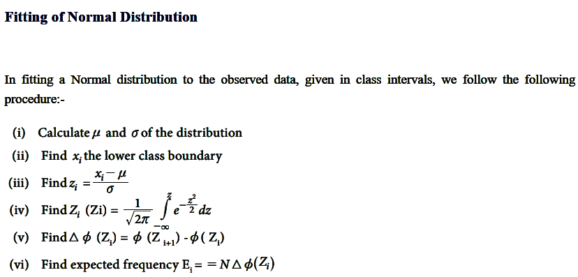
Characteristics Fitting a Normal Distribution

Poisson distribution is a probability distribution used to model the number of events occurring within a fixed interval of time, space, or other dimensions, given that these events occur independently and at a constant average rate.

Importance

1. Modeling Rare Events: Used to model the probability of rare events, such as accidents, machine failures, or phone call arrivals.
2. Applications in Various Fields: Applicable in business, biology, telecommunications, and reliability engineering.
3. Simplifies Complex Processes: Helps analyze situations with numerous trials and low probability of success per trial.
4. Foundation for Queuing Theory: Forms the basis for queuing models used in service and manufacturing industries.
5. Approximation of Binomial Distribution: When the number of trials is large, and the probability of success is small, Poisson distribution approximates the binomial distribution.

Conditions for Poisson Distribution

1. Independence: Events must occur independently of each other.
2. Constant Rate: The average rate (λ) of occurrence is constant over time or space.
3. Non-Simultaneous Events: Two events cannot occur simultaneously within the defined interval.
4. Fixed Interval: The observation is within a fixed time, space, or other defined intervals.

Constants

1. Mean (λ): Represents the expected number of events in the interval.
2. Variance (λ): Equal to the mean, reflecting the distribution’s spread.
3. Skewness: The distribution is skewed to the right when λ is small and becomes symmetric as λ increases.
4. Probability Mass Function (PMF): P(X = k) = [e^−λ*λ^k] / k!, Where $k$ is the number of occurrences, $e$ is the base of the natural logarithm, and λ is the mean.

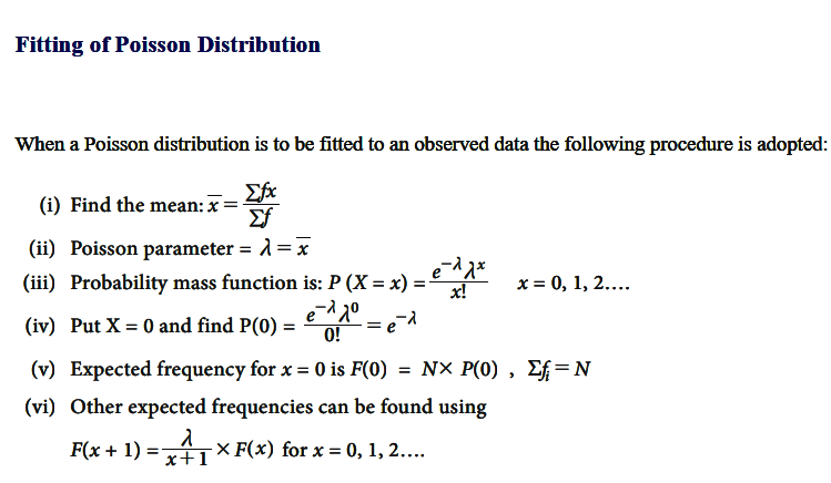
Fitting of Poisson Distribution

When a Poisson distribution is to be fitted to an observed data the following procedure is adopted: