Category: Bangalore University B.com Notes

According to the Negotiable Instruments Act 1881, “A bill of exchange is defined as an instrument in writing containing an unconditional order, signed by the maker, directing a certain person to pay a certain sum of money only to, or to the order of a certain person or to the bearer of the instrument.”

Features of bill of exchange

• It is important to have a bill of exchange in writing
• It must contain a confirm order to make a payment and not just the request
• The order should not have any condition
• The bill of exchange amount should be definite
• Fixed date for the amount to be paid
• The bill must be signed by both the drawee and the drawer
• The amount stated on the bill should be paid on-demand or on the expiry of a fixed time
• The amount is paid to the beneficiary of the bill, specific person, or against a definite order

Types of Bill of Exchange

1. Documentary Bill

In this, the bill of exchange is supported by the relevant documents that confirm the genuineness of sale or transaction that took place between the seller and buyer.

2. Demand Bill

This bill is payable when it demanded. The bill does not have a fixed date of payment, therefore, the bill has to be cleared whenever presented.

3. Usance Bill

It is a time-bound bill which means the payment has to be made within the given time period and time.

4. Inland Bill

An Inland bill is payable only in one country and not in any other foreign country. This bill is opposite to foreign bill.

5. Clean Bill

This bill does not have any proof of a document, so the interest is comparatively higher than the other bills.

6. Foreign Bill

A bill that can be paid outside India is termed as a foreign bill. Two examples of a foreign bill are an export bill and import bill.

7. Accommodation Bill

A bill that is sponsored, drawn, accepted without any condition is known as an accommodation bill.

8. Trade Bill

This kind of bill is specially related only to trade.

9. Supply Bill

The bill that is withdrawn by the supplier or contractor from the government department is known as the supply bill.

Advantages of Bill of Exchange

• Legal Document: It is a legal document, and if the drawee fails to make the payment it will be easier for the drawer to recover the amount legally.
• Discounting Facility: The bill bearer has to wait till the due date of the bill to receive the payment and it from the bank before its due date.
• Endorsement Possible: This bill of exchange can be exchanged from one individual to another for the adjustment of the debt.

Parties of Bill of Exchange

A bill of exchange has three parties:

1. Drawer

• The drawer is the maker of a bill of exchange.
• The bill is signed by Drawer.
• A creditor who is entitled to receive payment from the debtor can draw a bill of exchange.

2. Drawee

• Drawee is the person upon whom the bill of exchange is drawn.
• Drawee is the debtor who has to pay the money to the drawer.
• He is also known as ‘Acceptor’.

3. Payee

• The payee is the person to whom payment has to be made.
• The payee may be the drawer himself or a third party.

Importance of Promissory note in Bill of Exchange

According to the Negotiable Instruments Act 1881, the meaning of promissory note is ‘an instrument in writing (not being a banknote or a currency note), containing an unconditional undertaking signed by the maker, to pay a certain sum of money only to or to the order of a certain person, or to the bearer of the instrument. However, according to the Reserve Bank of India Act, a promissory note payable to bearer is illegal. Therefore, a promissory note cannot be made payable to the bearer.’

Crossing of a cheque is nothing but instructing the banker to pay the specified sum through the banker only, i.e. the amount on the cheque has to be deposited directly to the bank account of the payee.

Hence, it is not instantly encashed by the holder presenting the cheque at the bank counter. If any cheque contains such an instruction, it is called a crossed cheque.

The crossing of a cheque is done by making two transverse parallel lines at the top left corner across the face of the cheque.

Types of Crossing

The way a cheque is crossed specified the banker on how the funds are to be handled, to protect it from fraud and forgery. Primarily, it ensures that the funds must be transferred to the bank account only and not to encash it right away upon the receipt of the cheque. There are several types of crossing

1. General Crossing

When across the face of a cheque two transverse parallel lines are drawn at the top left corner, along with the words & Co., between the two lines, with or without using the words not negotiable. When a cheque is crossed in this way, it is called a general crossing.

2. Restrictive Crossing

When in between the two transverse parallel lines, the words ‘A/c payee’ is written across the face of the cheque, then such a crossing is called restrictive crossing or account payee crossing. In this case, the cheque can be credited to the account of the stated person only, making it a non-negotiable instrument.

3. Special Crossing

A cheque in which the name of the banker is written, across the face of the cheque in between the two transverse parallel lines, with or without using the word ‘not negotiable’. This type of crossing is called a special crossing. In a special crossing, the paying banker will pay the sum only to the banker whose name is stated in the cheque or to his agent. Hence, the cheque will be honoured only when the bank mentioned in the crossing orders the same.

4. Not Negotiable Crossing

When the words not negotiable is mentioned in between the two transverse parallel lines, indicating that the cheque can be transferred but the transferee will not be able to have a better title to the cheque.

5. Double Crossing

Double crossing is when a bank to whom the cheque crossed specially, further submits the same to another bank, for the purpose of collection as its agent, in this situation the second crossing should indicate that it is serving as an agent of the prior banker, to whom the cheque was specially crossed.

The crossing of a cheque is done to ensure the safety of payment. It is a well-known mechanism used to protect the parties to the cheque, by making sure that the payment is made to the right payee. Hence, it reduces fraud and wrong payments, as well as it protects the instrument from getting stolen or encashed by any unscrupulous individual.

Absolute skewness

This is obtained by finding the difference between any two measures of dispersion viz: Mean, Median and More. Thus, Skewness or

Any positive value obtained by any of the above formulae is marked as the extent of the positive skewness. Any negative value obtained by any of the above formulae is marked as the extent of the negative skewness of the distribution. If the result produced is zero, it signifies the absence of skewness in the distribution.

(a)    Co-efficient of skewness

 This is obtained by dividing the Skewness by any measure of dispersion.

Thus,

Karl Pearson’s Skewness

Prof. Karl pearson says that to study the skewness of a series, the difference between the Mean and Mode only should be found out. This is because, Mean is an average which is affected very much by the extreme values of a series and Mode is an average which is least affected by the extreme values of a series. Thus, according to him,

Sk_(p) = Mean –Mode

When, Mode is ill defined i.e. when it has different values, Prof. Pearson proposes to find out the skewness by the following formula:

Sk_(p) = 3 (Mean –Median)

This formula is based on the empirical relationship between Mean, Median and Mode which is as follows:

Absolute              Mode= 3 Median – 2 Mean

Thus,     Sk(p)      = X¯ – (3M- 2X¯)

                                =  X¯ – 3M +2X¯

                                = 3X¯ – 3M

                                = 3(X¯ -M)

For finding the coefficient of skewness, Prof. Pearson advocates that only standard diviation should be taken as the divisor of the absolute skewness. This is because, standard deviation is the only measure of dispersion which possesses many algebraic properties, and other measures of dispersion are not capable of algebraic treatments. Thus, his coefficient of skewness is given by:

Limits of the results

Prof. Pearson claims that the results of his coefficient of skewness shall lie withing ± 3.

Bowley’s Skewness

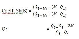
According to Prof. A.L. Bowley, the presence, or absence of skewness will be determined on the basis of the distance of the quartiles from the Median. Thus, his skewness is given by

                SK(B) = (Q₃ – M) – (M –Q₁)

                Or     = Q₃ + Q₁ -2M

If the above equation results in zero, it will indicate the absence of skewness or symmetricity of the distribution. On the other hand, if the said equation results in some positive, or negative figure, the same will be marked as the extent of the positive, or negative skewness of the series respectively.

Further, the coefficient, the coefficient of skewness of Prof. Bowley is given by:

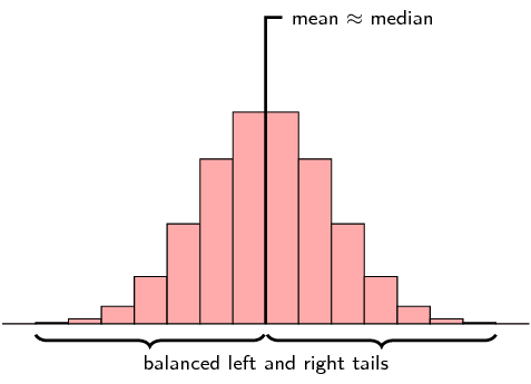
A symmetric distribution is one where the left and right hand sides of the distribution are roughly equally balanced around the mean. The histogram below shows a typical symmetric distribution.

For symmetric distributions, the mean is approximately equal to the median. The tails of the distribution are the parts to the left and to the right, away from the mean. The tail is the part where the counts in the histogram become smaller. For a symmetric distribution, the left and right tails are equally balanced, meaning that they have about the same length.

Symmetrical distribution occurs when the values of variables occur at regular frequencies and the mean, median and mode occur at the same point. In graph form, symmetrical distribution often appears as a bell curve. If a line were drawn dissecting the middle of the graph, it would show two sides that mirror each other. Symmetrical distribution is a core concept in technical trading as the price action of an asset is assumed to fit a symmetrical distribution curve over time.

Symmetrical distribution is used by traders to establish the value area for a stock, currency or commodity on a set time frame. This time frame is can be intraday, such as 30 minute intervals, or it can be longer-term using sessions or even weeks and months. A bell curve can be drawn around the price points hit during that time period and it is expected that most of the price action – approximately 68% of price points – will fall within one standard deviation of the centre of the curve. The curve is applied to the y-axis (price) as it is the variable whereas time throughout the period is simply linear. So the area within one standard deviation of the mean is the value area where price and the actual value of the asset are most closely matched.

If the price action takes the asset price out of the value area, then it suggests that price and value are out of alignment. If the breach is to the bottom of the curve, the asset is considered to be undervalued. If it is to the top of the curve, the asset is to be overvalued. The assumption is that the asset will revert to the mean over time.

An Example of How Symmetrical Distribution is Used

Symmetrical distribution is most often used to put price action into context. The further the price action wanders from the value area one standard deviation on each side of the mean, the greater the probability that the underlying asset is being under or overvalued by the market. This observation will suggest potential trades to place based on how far the price action has wandered from the mean for the time period being used. On larger time scales, however, there is a much greater risk of missing the actual entry and exit points.

• Symmetrical distribution can refer to a bell curve or any curve where a halving line produces mirror images.
• When traders speak of reversion to the mean, they are referring to the symmetrical distribution of price action overtime.
• The opposite of symmetrical distribution is asymmetrical distribution, which is a curve that exhibits skewness.

Skewed

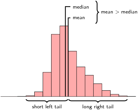
A distribution that is skewed right (also known as positively skewed) is shown below.

Now the picture is not symmetric around the mean anymore. For a right skewed distribution, the mean is typically greater than the median. Also notice that the tail of the distribution on the right hand (positive) side is longer than on the left hand side.

From the box and whisker diagram we can also see that the median is closer to the first quartile than the third quartile. The fact that the right hand side tail of the distribution is longer than the left can also be seen.

A distribution that is skewed left has exactly the opposite characteristics of one that is skewed right:

• The mean is typically less than the median;
• The tail of the distribution is longer on the left hand side than on the right hand side; and
• The median is closer to the third quartile than to the first quartile.

Measures of dispersion refer to statistical tools used to describe the spread or variability of a dataset. These measures help in understanding the extent to which data points differ from the central tendency (mean, median, or mode). Common measures of dispersion include:

• Range: The difference between the highest and lowest values.
• Variance: The average squared deviation of each data point from the mean.
• Standard deviation: The square root of variance, providing a more interpretable measure of spread.
• Interquartile range (IQR): The range between the 25th and 75th percentiles.

Characteristics of Measures of Dispersion:

• A measure of dispersion should be rigidly defined
• It must be easy to calculate and understand
• Not affected much by the fluctuations of observations
• Based on all observations

Classification of Measures of Dispersion

The measure of dispersion is categorized as:

(i) An absolute measure of dispersion:

• The measures which express the scattering of observation in terms of distances i.e., range, quartile deviation.
• The measure which expresses the variations in terms of the average of deviations of observations like mean deviation and standard deviation.

(ii) A relative measure of dispersion:

We use a relative measure of dispersion for comparing distributions of two or more data set and for unit free comparison. They are the coefficient of range, the coefficient of mean deviation, the coefficient of quartile deviation, the coefficient of variation, and the coefficient of standard deviation.

Coefficient of Dispersion

Whenever we want to compare the variability of the two series which differ widely in their averages. Also, when the unit of measurement is different. We need to calculate the coefficients of dispersion along with the measure of dispersion. The coefficients of dispersion (C.D.) based on different measures of dispersion are

• Based on Range = (X _max – X _min) ⁄ (X _max + X _min).
• C.D. based on quartile deviation = (Q₃ – Q1) ⁄ (Q₃ + Q1).
• Based on mean deviation = Mean deviation/average from which it is calculated.
• For Standard deviation = S.D. ⁄ Mean

Coefficient of Variation

100 times the coefficient of dispersion based on standard deviation is the coefficient of variation (C.V.).

C.V. = 100 × (S.D. / Mean) = (σ/ȳ ) × 100

Probable Error is basically the correlation coefficient that is fully responsible for the value of the coefficients and its accuracy.

As mentioned, probable error is the coefficient of correlation that supports in finding out about the accurate values of the coefficients. It also helps in determining the reliability of the coefficient.

The calculation of the correlation coefficient usually takes place from the samples. These samples are in pairs. The pairs generally come from a very large population. It is quite an easy job to find out about the limits and bounds of the correlation coefficient.

The correlation coefficient for a population is usually based on the knowledge and the sample relating to the correlation coefficient. Therefore, probable error is the easy way to find out or obtain the correlation coefficient of any population. Hence, the definition is:

Probable Error = 0.674 × 1−r2√N

Here, r = correlation coefficient of ‘n’ pairs of observations for any random sample and N = Total number of observations.

About the Values

• There is hardly any correlation between the different variables if the value of ‘r’ turns out to be less than the value of the probable error
• The value of correlation coefficient is generally certain if and only if the value of ‘r’ is around 6 times more than the value of the error.
•  The value of the probable error is in the bounds -1 and +1(-1≤r≤1). So, we can express it in the following manner.

Probable Limit

To get the upper limit and the lower limit, all we need to do is respectively add and subtract the value of probable error from the value of ‘r.’ This is exactly where the value of correlation of coefficient lies.

ρ (rho) = r ± P.E.

Here, the value of rho is nothing but the correlation coefficient of a population. This is also the limit of the correlation of coefficient. Alongside,

Probable Error = 2/3 SE

Here, S.E is Standard Error of Correlation Coefficient

Standard Error = (1-r²)/√N

Standard Error is basically the standard deviation of any mean. It is the sampling distribution of the standard deviation. The standard error is generally used to refer to any sort of estimate belonging to the standard deviation. Therefore, we use probable error to calculate and check the reliability associated with the coefficient.

Advantages of Standard Error

• It helps in finding and reducing the sample errors as well as the measurement errors.
• The standard error of any mean tells about the accuracy of the estimate clearly enough.

Formulas for Calculating Probable Error

Generally, there are three formulas using which we can calculate the probable error. The very first formula is the most common formula to calculate P.E. We use the Pearson product-moment method for calculating the same. It is:

P.E r  _{product-moment} = 0.6745(1-r²)/√N

The second formula is applicable when we need the probable error for rho. We use the Spearman method to calculate the value. The formula for the same is:

P.E. ρ = 0.6745(1-ρ²)/√N {1 + 1.086ρ² + 0.13ρ⁴ + .002ρ⁶}

The third formula is applicable to the Pearson coefficient ‘r.’  We calculate it through ρ by using the transmutation formula. The value is r = 2 sin (πρ/6). The formula is given by:

1. E  r_{found from ρ} = 0.7063 (1 – r²)√N {1 + 1.042r² + 0.008r⁴ + .002r⁶}

Note: The formula that we are using to calculate probable error is valid and applicable if the given population is normal.

Conditions to find Probable Error

We can find the probable error if and only if the given below conditions are taken care of.

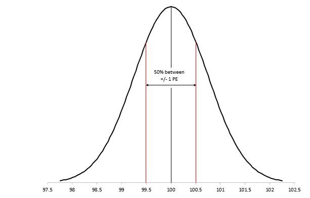
• The data that we have must be a bell-shaped curve. This means that the data has to give us a normal frequency curve
• It is important to take the probable error for measuring the statistics from the sample only
• It is compulsory that the sample items are taken off in an unbiased manner and must remain independent of each other’s value

We use this method of construction for computation of index price. As a result, the total cost of any commodity in any given year to the total cost of any commodity in the base year is in percentage form.

Simple Aggregative Price Index – (∑ P_n/ ∑ P₀) * 100

Where

∑P_n = Sum of the price of all the respective commodity in the current time period.
∑P_o = Sum of the price of all the respective commodity in the base period.

The simple aggregative index is very simple to understand. However, there is a serious defect in this method. The first commodity, here, has more influence than the rest two. This is so because the first commodity has a high price than the rest.

Furthermore, if we anyhow change the units, the index number will also go through a change. This is one of the biggest flaws of this methods. Use of absolute quantities turn the tables around. Therefore, considering independent values for the three years would be a better option.

To construct a simple price index, compute the price relatives and average them. Add the price relatives and divide them by the number of items. Table illustrates the construction of a simple index of wholesale prices.

Price index in 1980 = Prices in 1980 / Prices in 1970 x 100

Or ∑P₁/P₀ x 100 = 870/500 x 100 = 174

Using arithmetic mean, price index in 1980 = ∑R/N = 870/5 = 174

The preceding table shows that 1970 is the base period and 1980 is the year for which the price index has been constructed on the basis of price relatives. The index of wholesale prices in 1980 comes to 174. This means that the price level rose by 74 per cent in 1980 over 1970.

Consumer Price Index is also known as the cost of living index.

It represents the average change in price over a period of time, paid by a consumer for a fixed basket of goods and services.

Uses of CPI:

• It indicates the changes in the consumer prices.
• It evaluates the purchasing power of money.
• It is also used for comparison purposes.

Limitations of CPI;

• CPI focuses on a fixed basket, as consumer behaviour cannot be predicted, we can’t be very sure about CPI value to be relevant.
• Quality is not considered while calculating the CPI.
• Inflation effects are not taken into consideration as the basket is fixed.

CPI can be computed using 2 methods:

• Aggregate Expenditure method

CPI = (Total expenditure in current year/Total expenditure in base year)*100; which means;

CPI = Σp1q0/Σp0q0 * 100

• Family Budget method

CPI =  ΣWP/ ΣW

Where P = p1/p0 * 100

The frequency is the number of times an event occurs within a given scenario. Cumulative frequency is defined as the running total of frequencies. It is the sum of all the previous frequencies up to the current point. It is easily understandable through a Cumulative Frequency Table.

Cumulative Frequency is an important tool in Statistics to tabulate data in an organized manner. Whenever you wish to find out the popularity of a certain type of data, or the likelihood that a given event will fall within certain frequency distribution, a cumulative frequency table can be most useful. Say, for example, the Census department has collected data and wants to find out all residents in the city aged below 45. In this given case, a cumulative frequency table will be helpful.

Cumulative Frequency Curve

A curve that represents the cumulative frequency distribution of grouped data on a graph is called a Cumulative Frequency Curve or an Ogive. Representing cumulative frequency data on a graph is the most efficient way to understand the data and derive results.

There are two types of Cumulative Frequency Curves (or Ogives) :

• More than type Cumulative Frequency Curve
• Less than type Cumulative Frequency Curve

A frequency polygon is a graphical form of representation of data. It is used to depict the shape of the data and to depict trends. It is usually drawn with the help of a histogram but can be drawn without it as well. A histogram is a series of rectangular bars with no space between them and is used to represent frequency distributions.

Steps to Draw a Frequency Polygon

• Mark the class intervals for each class on the horizontal axis. We will plot the frequency on the vertical axis.
• Calculate the classmark for each class interval. The formula for class mark is:

Classmark = (Upper limit + Lower limit) / 2

• Mark all the class marks on the horizontal axis. It is also known as the mid-value of every class.
• Corresponding to each class mark, plot the frequency as given to you. The height always depicts the frequency. Make sure that the frequency is plotted against the class mark and not the upper or lower limit of any class.
• Join all the plotted points using a line segment. The curve obtained will be kinked.
• This resulting curve is called the frequency polygon.

Note that the above method is used to draw a frequency polygon without drawing a histogram. You can also draw a histogram first by drawing rectangular bars against the given class intervals. After this, you must join the midpoints of the bars to obtain the frequency polygon. Remember that the bars will have no spaces between them in a histogram.

Question 1: Construct a frequency polygon using the data given below:

Answer: We first need to calculate the cumulate frequency from the frequency given.

We now start by plotting the class marks such as 54.5, 64.5, 74.5 and so on till 94.5. Note that we will also plot the previous and next class marks to start and end the polygon, i.e. we plot 44.5 and 104.5 as well.

Then, the frequencies corresponding to the class marks are plotted against each class mark. Like you can see below, this makes sense as the frequency for class marks 44.5 and 104.5 are zero and touching the x-axis. These plot points are used only to give a closed shape to the polygon. The polygon looks like this: