Tag: Risk Analysis

Simple Average or Price Relatives Method

In this method, we find out the price relative of individual items and average out the individual values. Price relative refers to the percentage ratio of the value of a variable in the current year to its value in the year chosen as the base.

Price relative (R) = (P1÷P2) × 100

Here, P1= Current year value of item with respect to the variable and P2= Base year value of the item with respect to the variable. Effectively, the formula for index number according to this method is:

 P = ∑[(P1÷P2) × 100] ÷N

Here, N= Number of goods and P= Index number.

Weighted index method

Weighted Aggregate Method

Here different goods are assigned weight according to the quantity bought. There are three well-known sub-methods based on the different views of economists as mentioned below:

Laspeyre’s Method

Laspeyre was of the view that base year quantities must be chosen as weights. Therefore the formula is :

P = (∑P₁Q₀÷∑P₀Q₀)×100

Here,  ∑P₁Q₀= Summation of prices of current year multiplied by quantities of the base year taken as weights and ∑P₀Q₀= Summation of, prices of base year multiplied by quantities of the base year taken as weights.

Paasche Index Number

The Paasche Price Index is a consumer price index used to measure the change in the price and quantity of a basket of goods and services relative to a base year price and observation year quantity. Developed by German economist Hermann Paasche, the Paasche Price Index is commonly referred to as the “current weighted index.”

Formula for the Paasche Price Index

The formula for the index is as follows:

Where:

• Pi,0 is the price of the individual item at the base period and Pi,t is the price of the individual item at the observation period.
• Qi,t is the quantity of the individual item at the observation period.

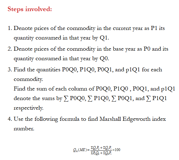
Marshall Edgeworth Index Number

Skewness, in statistics, is the degree of distortion from the symmetrical bell curve, or normal distribution, in a set of data. Skewness can be negative, positive, zero or undefined. A normal distribution has a skew of zero, while a lognormal distribution, for example, would exhibit some degree of right-skew.

The three probability distributions depicted below depict increasing levels of right (or positive) skewness. Distributions can also be left (negative) skewed. Skewness is used along with kurtosis to better judge the likelihood of events falling in the tails of a probability distribution.

Right skewness

• Skewness, in statistics, is the degree of distortion from the symmetrical bell curve in a probability distribution.
• Distributions can exhibit right (positive) skewness or left (negative) skewness to varying degree.
• Investors note skewness when judging a return distribution because it, like kurtosis, considers the extremes of the data set rather than focusing solely on the average.

Broadly speaking, there are two types of skewness: They are

(1) Positive skewness

(2) Negative skewnes.

Positive skewness

A series is said to have positive skewness when the following characteristics are noticed:

• Mean > Median > Mode.
• The right tail of the curve is longer than its left tail, when the data are plotted through a histogram, or a frequency polygon.
• The formula of Skewness and its coefficient give positive figures.

Negative Skewness

A series is said to have negative skewness when the following characteristics are noticed:

• Mode> Median > Mode.
• The left tail of the curve is longer than the right tail, when the data are plotted through a histogram, or a frequency polygon.
• The formula of skewness and its coefficient give negative figures.

Thus, a statistical distribution may be three types viz.

• Symmetric
• Positively skewed
• Negatively skewed

Skewness Co-efficient

1. Pearson’s Coefficient of Skewness #1 uses the mode. The formula is:

   

   Where  = the mean, Mo = the mode and s = the standard deviation for the sample.

2. Pearson’s Coefficient of Skewness #2 uses the median. The formula is:

   

   Where  = the mean, Mo = the mode and s = the standard deviation for the sample.

   It is generally used when you don’t know the mode.