Perpetuity, Function

Perpetuity refers to a financial instrument or cash flow that continues indefinitely without an end. In simpler terms, it is a stream of cash flows that occurs at regular intervals for an infinite duration. The present value of a perpetuity can be calculated using the formula:

PV = C/ r

Where,

C is the cash flow per period

r is the discount rate.

The concept of perpetuity has several important functions in finance and investment analysis. Here are eight key functions of perpetuity:

  • Valuation of Investments:

Perpetuity provides a method for valuing investments that generate constant cash flows over an indefinite period. This is particularly useful in valuing companies, real estate, and other assets that are expected to generate steady income streams indefinitely. By calculating the present value of these cash flows, investors can determine the fair value of such assets.

  • Determining Fixed Income Securities:

Perpetuities are often used in valuing fixed income securities like preferred stocks and bonds that pay a constant dividend or interest indefinitely. Investors can assess the attractiveness of these securities by comparing their present value to the market price, thus aiding investment decisions.

  • Simplifying Financial Analysis:

The concept of perpetuity simplifies complex financial models by allowing analysts to consider cash flows that extend indefinitely. This simplification is particularly valuable in scenarios where cash flows are expected to remain constant over a long period, providing a clearer picture of an investment’s worth.

  • Corporate Valuation:

In corporate finance, perpetuity is a critical component of valuation models, such as the Gordon Growth Model, which estimates the value of a company based on its expected future dividends. By considering dividends as a perpetuity, analysts can derive a more accurate valuation for firms with stable dividend policies.

  • Real Estate Investment:

In real estate, perpetuity helps in evaluating properties that generate consistent rental income. Investors can use the perpetuity formula to estimate the present value of future rental cash flows, facilitating better decision-making regarding property purchases or investments.

  • Retirement Planning:

Perpetuity can assist individuals in planning for retirement. By understanding how much they can withdraw from their retirement savings while maintaining a sustainable income level indefinitely, retirees can ensure financial security throughout their retirement years.

  • Life Insurance Valuation:

Perpetuities play a role in life insurance products that provide lifelong benefits. The present value of future benefits can be calculated using the perpetuity concept, aiding insurers in pricing their products and ensuring they can meet future obligations.

  • Evaluating Charitable Donations:

Nonprofit organizations can benefit from the concept of perpetuity when structuring endowments or perpetual funds. These funds are designed to provide a steady stream of income for ongoing operations, scholarships, or charitable initiatives. By understanding the present value of these perpetual cash flows, organizations can make informed decisions about resource allocation and fund management.

Business Quantitative Analysis 1st Semester BU B.Com SEP Notes

Unit 1,2,3,4 Pl. Refer Books Book


Unit 5 [Book]
Definition of Interest and Other Terms: Simple Interest and Compound Interest VIEW
Effective rate of Interest:
Present Value VIEW
Future Value VIEW
Perpetuity VIEW
Annuity VIEW
Sinking Fund VIEW
Valuation of Bonds VIEW
Calculating of EMI VIEW


Business Mathematics & Statistics Bangalore University B.com 3rd Semester NEP Notes

Unit 1 Commercial Arithmetic [Book]
Percentage VIEW
Cost, Profit and Selling price VIEW
Ratio Proportion VIEW
Problems on Speed and Time VIEW
Interest-Simple interest and Compound interest VIEW
Annuity VIEW


Unit 2 Theory of Equations [Book] No Update


Unit 3 Matrices and Determinants [Book] No Update


Unit 4 Measures of Central Tendency and Dispersion [Book]
Introduction Meaning and Definition, Objectives of measures of Central tendency VIEW
Types of averages: Arithmetic mean (Simple average only) VIEW
Median VIEW
Mode VIEW
Meaning and Objectives of measures of Dispersion VIEW
VIEW VIEW
Standard deviation and coefficient of Variation VIEW
Skewness VIEW VIEW
Problems on Direct method only VIEW


Unit 5 Correlation and Regression [Book]
Correlation: Meaning and definition-uses VIEW VIEW
VIEW
Karl Pearson’s coefficient of correlation (deviation from actual mean only) VIEW
Spearman’s Rank Correlation Coefficient VIEW
Regression Meaning VIEW
Regression Equations, Estimating x and y values VIEW
Finding correlation coefficient with Regression coefficient VIEW VIEW

Normal Distribution: Importance, Central Limit Theorem

Normal distribution, or the Gaussian distribution, is a fundamental probability distribution that describes how data values are distributed symmetrically around a mean. Its graph forms a bell-shaped curve, with most data points clustering near the mean and fewer occurring as they deviate further. The curve is defined by two parameters: the mean (μ) and the standard deviation (σ), which determine its center and spread. Normal distribution is widely used in statistics, natural sciences, and social sciences for analysis and inference.

The general form of its probability density function is:

The parameter μ is the mean or expectation of the distribution (and also its median and mode), while the parameter σ is its standard deviation. The variance of the distribution is σ^2. A random variable with a Gaussian distribution is said to be normally distributed, and is called a normal deviate.

Normal distributions are important in statistics and are often used in the natural and social sciences to represent real-valued random variables whose distributions are not known. Their importance is partly due to the central limit theorem. It states that, under some conditions, the average of many samples (observations) of a random variable with finite mean and variance is itself a random variable whose distribution converges to a normal distribution as the number of samples increases. Therefore, physical quantities that are expected to be the sum of many independent processes, such as measurement errors, often have distributions that are nearly normal.

A normal distribution is sometimes informally called a bell curve. However, many other distributions are bell-shaped (such as the Cauchy, Student’s t, and logistic distributions).

Importance of Normal Distribution:

  1. Foundation of Statistical Inference

The normal distribution is central to statistical inference. Many parametric tests, such as t-tests and ANOVA, are based on the assumption that the data follows a normal distribution. This simplifies hypothesis testing, confidence interval estimation, and other analytical procedures.

  1. Real-Life Data Approximation

Many natural phenomena and datasets, such as heights, weights, IQ scores, and measurement errors, tend to follow a normal distribution. This makes it a practical and realistic model for analyzing real-world data, simplifying interpretation and analysis.

  1. Basis for Central Limit Theorem (CLT)

The normal distribution is critical in understanding the Central Limit Theorem, which states that the sampling distribution of the sample mean approaches a normal distribution as the sample size increases, regardless of the population’s actual distribution. This enables statisticians to make predictions and draw conclusions from sample data.

  1. Application in Quality Control

In industries, normal distribution is widely used in quality control and process optimization. Control charts and Six Sigma methodologies assume normality to monitor processes and identify deviations or defects effectively.

  1. Probability Calculations

The normal distribution allows for the easy calculation of probabilities for different scenarios. Its standardized form, the z-score, simplifies these calculations, making it easier to determine how data points relate to the overall distribution.

  1. Modeling Financial and Economic Data

In finance and economics, normal distribution is used to model returns, risks, and forecasts. Although real-world data often exhibit deviations, normal distribution serves as a baseline for constructing more complex models.

Central limit theorem

In probability theory, the central limit theorem (CLT) establishes that, in many situations, when independent random variables are added, their properly normalized sum tends toward a normal distribution (informally a bell curve) even if the original variables themselves are not normally distributed. The theorem is a key concept in probability theory because it implies that probabilistic and statistical methods that work for normal distributions can be applicable to many problems involving other types of distributions. This theorem has seen many changes during the formal development of probability theory. Previous versions of the theorem date back to 1810, but in its modern general form, this fundamental result in probability theory was precisely stated as late as 1920, thereby serving as a bridge between classical and modern probability theory.

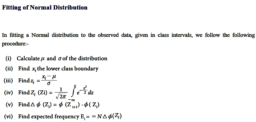
Characteristics Fitting a Normal Distribution

Poisson Distribution: Importance Conditions Constants, Fitting of Poisson Distribution

Poisson distribution is a probability distribution used to model the number of events occurring within a fixed interval of time, space, or other dimensions, given that these events occur independently and at a constant average rate.

Importance

  1. Modeling Rare Events: Used to model the probability of rare events, such as accidents, machine failures, or phone call arrivals.
  2. Applications in Various Fields: Applicable in business, biology, telecommunications, and reliability engineering.
  3. Simplifies Complex Processes: Helps analyze situations with numerous trials and low probability of success per trial.
  4. Foundation for Queuing Theory: Forms the basis for queuing models used in service and manufacturing industries.
  5. Approximation of Binomial Distribution: When the number of trials is large, and the probability of success is small, Poisson distribution approximates the binomial distribution.

Conditions for Poisson Distribution

  1. Independence: Events must occur independently of each other.
  2. Constant Rate: The average rate (λ) of occurrence is constant over time or space.
  3. Non-Simultaneous Events: Two events cannot occur simultaneously within the defined interval.
  4. Fixed Interval: The observation is within a fixed time, space, or other defined intervals.

Constants

  1. Mean (λ): Represents the expected number of events in the interval.
  2. Variance (λ): Equal to the mean, reflecting the distribution’s spread.
  3. Skewness: The distribution is skewed to the right when λ is small and becomes symmetric as λ increases.
  4. Probability Mass Function (PMF): P(X = k) = [e^−λ*λ^k] / k!, Where is the number of occurrences, is the base of the natural logarithm, and λ is the mean.

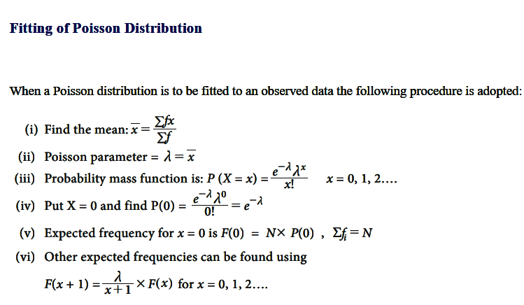
Fitting of Poisson Distribution

When a Poisson distribution is to be fitted to an observed data the following procedure is adopted:

Binomial Distribution: Importance Conditions, Constants

The binomial distribution is a probability distribution that summarizes the likelihood that a value will take one of two independent values under a given set of parameters or assumptions. The underlying assumptions of the binomial distribution are that there is only one outcome for each trial, that each trial has the same probability of success, and that each trial is mutually exclusive, or independent of each other.

In probability theory and statistics, the binomial distribution with parameters n and p is the discrete probability distribution of the number of successes in a sequence of n independent experiments, each asking a yes, no question, and each with its own Boolean-valued outcome: success (with probability p) or failure (with probability q = 1 − p). A single success/failure experiment is also called a Bernoulli trial or Bernoulli experiment, and a sequence of outcomes is called a Bernoulli process; for a single trial, i.e., n = 1, the binomial distribution is a Bernoulli distribution. The binomial distribution is the basis for the popular binomial test of statistical significance.

The binomial distribution is frequently used to model the number of successes in a sample of size n drawn with replacement from a population of size N. If the sampling is carried out without replacement, the draws are not independent and so the resulting distribution is a hypergeometric distribution, not a binomial one. However, for N much larger than n, the binomial distribution remains a good approximation, and is widely used

The binomial distribution is a common discrete distribution used in statistics, as opposed to a continuous distribution, such as the normal distribution. This is because the binomial distribution only counts two states, typically represented as 1 (for a success) or 0 (for a failure) given a number of trials in the data. The binomial distribution, therefore, represents the probability for x successes in n trials, given a success probability p for each trial.

Binomial distribution summarizes the number of trials, or observations when each trial has the same probability of attaining one particular value. The binomial distribution determines the probability of observing a specified number of successful outcomes in a specified number of trials.

The binomial distribution is often used in social science statistics as a building block for models for dichotomous outcome variables, like whether a Republican or Democrat will win an upcoming election or whether an individual will die within a specified period of time, etc.

Importance

For example, adults with allergies might report relief with medication or not, children with a bacterial infection might respond to antibiotic therapy or not, adults who suffer a myocardial infarction might survive the heart attack or not, a medical device such as a coronary stent might be successfully implanted or not. These are just a few examples of applications or processes in which the outcome of interest has two possible values (i.e., it is dichotomous). The two outcomes are often labeled “success” and “failure” with success indicating the presence of the outcome of interest. Note, however, that for many medical and public health questions the outcome or event of interest is the occurrence of disease, which is obviously not really a success. Nevertheless, this terminology is typically used when discussing the binomial distribution model. As a result, whenever using the binomial distribution, we must clearly specify which outcome is the “success” and which is the “failure”.

The binomial distribution model allows us to compute the probability of observing a specified number of “successes” when the process is repeated a specific number of times (e.g., in a set of patients) and the outcome for a given patient is either a success or a failure. We must first introduce some notation which is necessary for the binomial distribution model.

First, we let “n” denote the number of observations or the number of times the process is repeated, and “x” denotes the number of “successes” or events of interest occurring during “n” observations. The probability of “success” or occurrence of the outcome of interest is indicated by “p”.

The binomial equation also uses factorials. In mathematics, the factorial of a non-negative integer k is denoted by k!, which is the product of all positive integers less than or equal to k. For example,

  • 4! = 4 x 3 x 2 x 1 = 24,
  • 2! = 2 x 1 = 2,
  • 1!=1.
  • There is one special case, 0! = 1.

Conditions

  • The number of observations n is fixed.
  • Each observation is independent.
  • Each observation represents one of two outcomes (“success” or “failure”).
  • The probability of “success” p is the same for each outcome

Constants

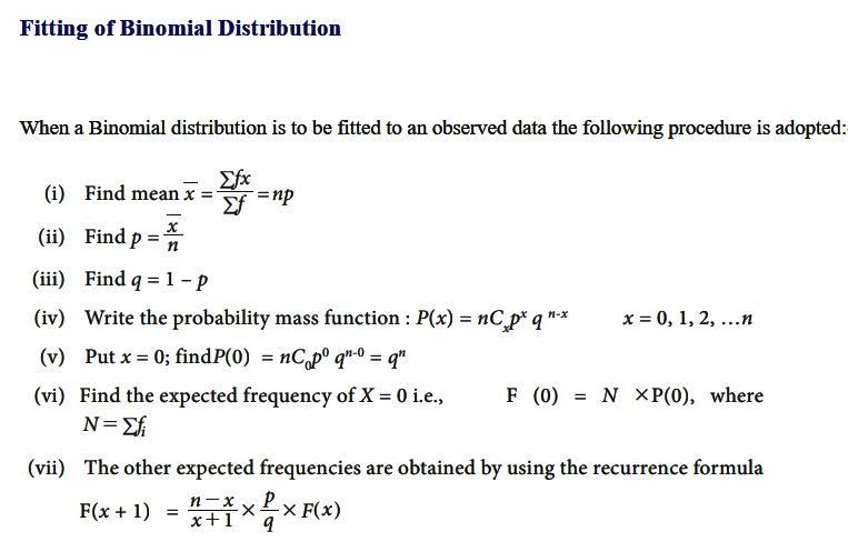
Fitting of Binomial Distribution

Fitting of probability distribution to a series of observed data helps to predict the probability or to forecast the frequency of occurrence of the required variable in a certain desired interval.

To fit any theoretical distribution, one should know its parameters and probability distribution. Parameters of Binomial distribution are n and p. Once p and n are known, binomial probabilities for different random events and the corresponding expected frequencies can be computed. From the given data we can get n by inspection. For binomial distribution, we know that mean is equal to np hence we can estimate p as = mean/n. Thus, with these n and p one can fit the binomial distribution.

There are many probability distributions of which some can be fitted more closely to the observed frequency of the data than others, depending on the characteristics of the variables. Therefore, one needs to select a distribution that suits the data well.

Calculation of Interest

Calculating interest rate is not at all a difficult method to understand. Knowing to calculate interest rate can solve a lot of wages problems and save money while taking investment decisions. There is an easy formula to calculate simple interest rates. If you are aware of your loan and interest amount you can pay, you can do the largest interest rate calculation for yourself.

Using the simple interest calculation formula, you can also see your interest payments in a year and calculate your annual percentage rate.

Here is the step by step guide to calculate the interest rate.

How to calculate interest rate?

Know the formula which can help you to calculate your interest rate.

Step 1

To calculate your interest rate, you need to know the interest formula I/Pt = r to get your rate. Here,

I = Interest amount paid in a specific time period (month, year etc.)

P = Principle amount (the money before interest)

t = Time period involved

r = Interest rate in decimal

You should remember this equation to calculate your basic interest rate.

Step 2

Once you put all the values required to calculate your interest rate, you will get your interest rate in decimal. Now, you need to convert the interest rate you got by multiplying it by 100. For example, a decimal like .11 will not help much while figuring out your interest rate. So, if you want to find your interest rate for .11, you have to multiply .11 with 100 (.11 x 100).

For this case, your interest rate will be (.11 x 100 = 11) 11%.

Step 3

Apart from this, you can also calculate your time period involved, principal amount and interest amount paid in a specific time period if you have other inputs available with you.

Calculate interest amount paid in a specific time period, I = Prt.

Calculate the principal amount, P = I/rt.

Calculate time period involved t = I/Pr.

Step 4

Most importantly, you have to make sure that your time period and interest rate are following the same parameter.

For example, on a loan, you want to find your monthly interest rate after one year. In this case, if you put t = 1, you will get the final interest rate as the interest rate per year. Whereas, if you want the monthly interest rate, you have to put the correct amount of time elapsed. Here, you can consider the time period like 12 months.

Please remember, your time period should be the same time amount as the interest paid. For example, if you’re calculating a year’s monthly interest payments then, it can be considered you’ve made 12 payments.

Also, you have to make sure that you check the time period (weekly, monthly, yearly etc.) when your interest is calculated with your bank.

Step 5

You can rely on online calculators to get interest rates for complex loans, such as mortgages. You should also know the interest rate of your loan when you sign up for it.

For fluctuating rates, sometimes it becomes difficult to determine what a certain rate means. So, it is better to use free online calculators by searching “variable APR interest calculator”, “mortgage interest calculator” etc.

Calculation of interest when rate of interest and cash price is given

  • Where Cash Price, Interest Rate and Instalment are Given:

Illustration:

On 1st January 2003, A bought a television from a seller under Hire Purchase System, the cash price of which being Rs 10.450 as per the following terms:

(a) Rs 3,000 to be paid on signing the agreement.

(b) Balance to be paid in three equal installments of Rs 3,000 at the end of each year,

(c) The rate of interest charged by the seller is 10% per annum.

You are required to calculate the interest paid by the buyer to the seller each year.

Solution:

Note:

  1. there is no time gap between the signing of the agreement and the cash down payment of Rs 3,000 (1.1.2003). Hence no interest is calculated. The entire amount goes to reduce the cash price.
  2. The interest in the last installment is taken at the differential figure of Rs 285.50 (3,000 – 2,714.50).

(2) Where Cash Price and Installments are Given but Rate of Interest is Omitted:

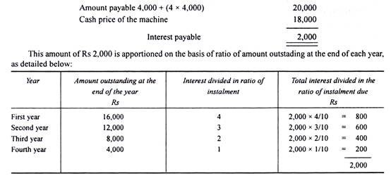
Where the rate of interest is not given and only the cash price and the total payments under hire purchase installments are given, then the total interest paid is the difference between the cash price of the asset and the total amount paid as per the agreement. This interest amount is apportioned in the ratio of amount outstanding at the end of each period.

Illustration:

Mr. A bought a machine under hire purchase agreement, the cash price of the machine being Rs 18,000. As per the terms, the buyer has to pay Rs 4,000 on signing the agreement and the balance in four installments of Rs 4,000 each, payable at the end of each year. Calculate the interest chargeable at the end of each year.
(3) Where installments and Rate of Interest are Given but Cash Value of the Asset is Omitted:

In certain problems, the cash price is not given. It is necessary that we must first find out the cash price and interest included in the installments. The asset account is to be debited with the actual price of the asset. Under such situations, i.e. in the absence of cash price, the interest is calculated from the last year.

It may be noted that the amount of interest goes on increasing from 3rd year to 2nd year, 2nd year to 1st year. Since the interest is included in the installments and by knowing the rate of interest, we can find out the cash price.

Thus:

Let the cash price outstanding be: Rs 100

Interest @ 10% on Rs 100 for a year: Rs 10

Installment paid at the end of the year 110

The interest on installment price = 10/110 or 1/11 as a ratio.

Illustration:

I buy a television on Hire Purchase System.

The terms of payment are as follows:

Rs 2,000 to be paid on signing the agreement;

Rs 2,800 at the end of the first year;

Rs 2,600 at the end of the second year;

Rs 2,400 at the end of the third year;

Rs 2,200 at the end of the fourth year.

If interest is charged at the rate of 10% p.a., what was the cash value of the television?

Solution:

(4) Calculation of Cash Price when Reference to Annuity Table, the Rate of Interest and Installments are Given:

Sometimes in the problem a reference to annuity table wherein present value of the annuity for a number of years at a certain rate of interest is given. In such cases the cash price is calculated by multiplying the amount of installment and adding the product to the initial payment.

Illustration:

A agrees to purchase a machine from a seller under Hire Purchase System by annual installment of Rs 10,000 over a period of 5 years. The seller charges interest at 4% p.a. on yearly balance.

N.B. The present value of Re 1 p.a. for five years at 4% is Rs 4.4518. Find out the cash price of the machine.

Solution:

Installment Re 1 Present value = Rs 4.4518

Installment = Rs 10,000 Present value = Rs 4.4518 x 10,000 = Rs 44,518

Credit: https://www.yourarticlelibrary.com/accounting/hire-purchase/how-to-calculate-interest-4-cases-hire-purchase/51175

Quantitative Methods for Business – 1

Unit 1 Number System {Book}

Natural Numbers, Even Numbers, Odd Numbers

VIEW

Integers, Prime Numbers

VIEW

Rational & Irrational numbers

VIEW

Real Numbers, HCF & LCM (Simple Problems)

VIEW

Unit 2 Theory Of Equations {Book}

Please refer Books for this Unit

VIEW

Unit 3 Progressions {Book}

Arithmetic Progression Finding the “n”th term of AP and Sum to “n”th term of AP.

VIEW

Insertion of Arithmetic Mean

VIEW

Geometric Progression Finding the “n”th term of GP and

VIEW

Insertion of Geometric Mean

VIEW

Unit 4 Matrices and Determinants {Book}

Please refer Books for this Unit

VIEW

Unit 4 Commercial Arithmetic {Book}

Simple Interest, Compound Interest including half yearly and quarterly calculations

VIEW

Annuities

VIEW

Percentages

VIEW

Bills Discounting

VIEW

Ratios and proportions

VIEW

Duplicate: Triplicate and Sub-duplicate of a ratio

VIEW

Proportions: Third, Fourth and inverse proportion

VIEW

Unit 5 Progressions {Book}

Arithmetic Progression Finding the “n”th term of AP and Sum to “n”th term of AP.

VIEW

Insertion of Arithmetic Mean

VIEW

Geometric Progression Finding the “n”th term of GP and

VIEW

Insertion of Geometric Mean

VIEW

Determinants of the Value of Bonds

Bonds are fixed-income securities that represent a loan from an investor to a borrower, typically a corporation or government. When purchasing a bond, the investor lends money in exchange for periodic interest payments and the return of the bond’s face value at maturity. Bonds are used to finance various projects and operations, providing a predictable income stream for investors.

Valuation of Bonds

The method for valuation of bonds involves three steps as follows:

Step 1: Estimate the expected cash flows

Step 2: Determine the appropriate interest rate that should be used to discount the cash flows.

& Step 3: Calculate the present value of the expected cash flows (step-1) using appropriate interest rate (step- 2) i.e. discounting the expected cash flows

Step 1: Estimating cash flows

Cash flow is the cash that is estimated to be received in future from investment in a bond. There are only two types of cash flows that can be received from investment in bonds i.e. coupon payments and principal payment at maturity.

The usual cash flow cycle of the bond is coupon payments are received at regular intervals as per the bond agreement, and final coupon plus principle payment is received at the maturity. There are some instances when bonds don’t follow these regular patterns. Unusual patterns maybe a result of the different type of bond such as zero-coupon bonds, in which there are no coupon payments. Considering such factors, it is important for an analyst to estimate accurate cash flow for the purpose of bond valuation.

Step 2: Determine the appropriate interest rate to discount the cash flows

Once the cash flow for the bond is estimated, the next step is to determine the appropriate interest rate to discount cash flows. The minimum interest rate that an investor should require is the interest available in the marketplace for default-free cash flow. Default-free cash flows are cash flows from debt security which are completely safe and has zero chances default. Such securities are usually issued by the central bank of a country, for example, in the USA it is bonds by U.S. Treasury Security.

Consider a situation where an investor wants to invest in bonds. If he is considering to invest corporate bonds, he is expecting to earn higher return from these corporate bonds compared to rate of returns of U.S. Treasury Security bonds. This is because chances are that a corporate bond might default, whereas the U.S. Security Treasury bond is never going to default. As he is taking a higher risk by investing in corporate bonds, he expects a higher return.

One may use single interest rate or multiple interest rates for valuation.

Step 3: Discounting the expected cash flows

Now that we already have values of expected future cash flows and interest rate used to discount the cash flow, it is time to find the present value of cash flows. Present Value of a cash flow is the amount of money that must be invested today to generate a specific future value. The present value of a cash flow is more commonly known as discounted value.

The present value of a cash flow depends on two determinants:

  • When a cash flow will be received i.e. timing of a cash flow &;
  • The required interest rate, more widely known as Discount Rate (rate as per Step-2)

First, we calculate the present value of each expected cash flow. Then we add all the individual present values and the resultant sum is the value of the bond.

The formula to find the present value of one cash flow is:

Present value formula for Bond Valuation

Present Value n = Expected cash flow in the period n/ (1+i) n

Here,

i = rate of return/discount rate on bond
n = expected time to receive the cash flow

By this formula, we will get the present value of each individual cash flow t years from now. The next step is to add all individual cash flows.

Bond Value = Present Value 1 + Present Value 2 + ……. + Present Value n

Sampling and Sampling Distribution

Sample design is the framework, or road map, that serves as the basis for the selection of a survey sample and affects many other important aspects of a survey as well. In a broad context, survey researchers are interested in obtaining some type of information through a survey for some population, or universe, of interest. One must define a sampling frame that represents the population of interest, from which a sample is to be drawn. The sampling frame may be identical to the population, or it may be only part of it and is therefore subject to some under coverage, or it may have an indirect relationship to the population.

Sampling is the process of selecting a subset of individuals, items, or observations from a larger population to analyze and draw conclusions about the entire group. It is essential in statistics when studying the entire population is impractical, time-consuming, or costly. Sampling can be done using various methods, such as random, stratified, cluster, or systematic sampling. The main objectives of sampling are to ensure representativeness, reduce costs, and provide timely insights. Proper sampling techniques enhance the reliability and validity of statistical analysis and decision-making processes.

Steps in Sample Design

While developing a sampling design, the researcher must pay attention to the following points:

  • Type of Universe:

The first step in developing any sample design is to clearly define the set of objects, technically called the Universe, to be studied. The universe can be finite or infinite. In finite universe the number of items is certain, but in case of an infinite universe the number of items is infinite, i.e., we cannot have any idea about the total number of items. The population of a city, the number of workers in a factory and the like are examples of finite universes, whereas the number of stars in the sky, listeners of a specific radio programme, throwing of a dice etc. are examples of infinite universes.

  • Sampling unit:

A decision has to be taken concerning a sampling unit before selecting sample. Sampling unit may be a geographical one such as state, district, village, etc., or a construction unit such as house, flat, etc., or it may be a social unit such as family, club, school, etc., or it may be an individual. The researcher will have to decide one or more of such units that he has to select for his study.

  • Source list:

It is also known as ‘sampling frame’ from which sample is to be drawn. It contains the names of all items of a universe (in case of finite universe only). If source list is not available, researcher has to prepare it. Such a list should be comprehensive, correct, reliable and appropriate. It is extremely important for the source list to be as representative of the population as possible.

  • Size of Sample:

This refers to the number of items to be selected from the universe to constitute a sample. This a major problem before a researcher. The size of sample should neither be excessively large, nor too small. It should be optimum. An optimum sample is one which fulfills the requirements of efficiency, representativeness, reliability and flexibility. While deciding the size of sample, researcher must determine the desired precision as also an acceptable confidence level for the estimate. The size of population variance needs to be considered as in case of larger variance usually a bigger sample is needed. The size of population must be kept in view for this also limits the sample size. The parameters of interest in a research study must be kept in view, while deciding the size of the sample. Costs too dictate the size of sample that we can draw. As such, budgetary constraint must invariably be taken into consideration when we decide the sample size.

  • Parameters of interest:

In determining the sample design, one must consider the question of the specific population parameters which are of interest. For instance, we may be interested in estimating the proportion of persons with some characteristic in the population, or we may be interested in knowing some average or the other measure concerning the population. There may also be important sub-groups in the population about whom we would like to make estimates. All this has a strong impact upon the sample design we would accept.

  • Budgetary constraint:

Cost considerations, from practical point of view, have a major impact upon decisions relating to not only the size of the sample but also to the type of sample. This fact can even lead to the use of a non-probability sample.

  • Sampling procedure:

Finally, the researcher must decide the type of sample he will use i.e., he must decide about the technique to be used in selecting the items for the sample. In fact, this technique or procedure stands for the sample design itself. There are several sample designs (explained in the pages that follow) out of which the researcher must choose one for his study. Obviously, he must select that design which, for a given sample size and for a given cost, has a smaller sampling error.

Types of Samples

  • Probability Sampling (Representative samples)

Probability samples are selected in such a way as to be representative of the population. They provide the most valid or credible results because they reflect the characteristics of the population from which they are selected (e.g., residents of a particular community, students at an elementary school, etc.). There are two types of probability samples: random and stratified.

  • Random Sample

The term random has a very precise meaning. Each individual in the population of interest has an equal likelihood of selection. This is a very strict meaning you can’t just collect responses on the street and have a random sample.

The assumption of an equal chance of selection means that sources such as a telephone book or voter registration lists are not adequate for providing a random sample of a community. In both these cases there will be a number of residents whose names are not listed. Telephone surveys get around this problem by random-digit dialling but that assumes that everyone in the population has a telephone. The key to random selection is that there is no bias involved in the selection of the sample. Any variation between the sample characteristics and the population characteristics is only a matter of chance.

  • Stratified Sample

A stratified sample is a mini-reproduction of the population. Before sampling, the population is divided into characteristics of importance for the research. For example, by gender, social class, education level, religion, etc. Then the population is randomly sampled within each category or stratum. If 38% of the population is college-educated, then 38% of the sample is randomly selected from the college-educated population.

Stratified samples are as good as or better than random samples, but they require fairly detailed advance knowledge of the population characteristics, and therefore are more difficult to construct.

  • Non-probability Samples (Non-representative samples)

As they are not truly representative, non-probability samples are less desirable than probability samples. However, a researcher may not be able to obtain a random or stratified sample, or it may be too expensive. A researcher may not care about generalizing to a larger population. The validity of non-probability samples can be increased by trying to approximate random selection, and by eliminating as many sources of bias as possible.

  • Quota Sample

The defining characteristic of a quota sample is that the researcher deliberately sets the proportions of levels or strata within the sample. This is generally done to insure the inclusion of a particular segment of the population. The proportions may or may not differ dramatically from the actual proportion in the population. The researcher sets a quota, independent of population characteristics.

Example: A researcher is interested in the attitudes of members of different religions towards the death penalty. In Iowa a random sample might miss Muslims (because there are not many in that state). To be sure of their inclusion, a researcher could set a quota of 3% Muslim for the sample. However, the sample will no longer be representative of the actual proportions in the population. This may limit generalizing to the state population. But the quota will guarantee that the views of Muslims are represented in the survey.

  • Purposive Sample

A purposive sample is a non-representative subset of some larger population, and is constructed to serve a very specific need or purpose. A researcher may have a specific group in mind, such as high level business executives. It may not be possible to specify the population they would not all be known, and access will be difficult. The researcher will attempt to zero in on the target group, interviewing whoever is available.

  • Convenience Sample

A convenience sample is a matter of taking what you can get. It is an accidental sample. Although selection may be unguided, it probably is not random, using the correct definition of everyone in the population having an equal chance of being selected. Volunteers would constitute a convenience sample.

Non-probability samples are limited with regard to generalization. Because they do not truly represent a population, we cannot make valid inferences about the larger group from which they are drawn. Validity can be increased by approximating random selection as much as possible, and making every attempt to avoid introducing bias into sample selection.

Sampling Distribution

Sampling Distribution is a statistical concept that describes the probability distribution of a given statistic (e.g., mean, variance, or proportion) derived from repeated random samples of a specific size taken from a population. It plays a crucial role in inferential statistics, providing the foundation for making predictions and drawing conclusions about a population based on sample data.

Concepts of Sampling Distribution

A sampling distribution is the distribution of a statistic (not raw data) over all possible samples of the same size from a population. Commonly used statistics include the sample mean (Xˉ\bar{X}), sample variance, and sample proportion.

Purpose:

It allows statisticians to estimate population parameters, test hypotheses, and calculate probabilities for statistical inference.

Shape and Characteristics:

    • The shape of the sampling distribution depends on the population distribution and the sample size.
    • For large sample sizes, the Central Limit Theorem states that the sampling distribution of the mean will be approximately normal, regardless of the population’s distribution.

Importance of Sampling Distribution

  • Facilitates Statistical Inference:

Sampling distributions are used to construct confidence intervals and perform hypothesis tests, helping to infer population characteristics.

  • Standard Error:

The standard deviation of the sampling distribution, called the standard error, quantifies the variability of the sample statistic. Smaller standard errors indicate more reliable estimates.

  • Links Population and Samples:

It provides a theoretical framework that connects sample statistics to population parameters.

Types of Sampling Distributions

  • Distribution of Sample Means:

Shows the distribution of means from all possible samples of a population.

  • Distribution of Sample Proportions:

Represents the proportion of a certain outcome in samples, used in binomial settings.

  • Distribution of Sample Variances:

Explains the variability in sample data.

Example

Consider a population of students’ test scores with a mean of 70 and a standard deviation of 10. If we repeatedly draw random samples of size 30 and calculate the sample mean, the distribution of those means forms the sampling distribution. This distribution will have a mean close to 70 and a reduced standard deviation (standard error).

error: Content is protected !!