Range and co-efficient of Range

The range is a measure of dispersion that represents the difference between the highest and lowest values in a dataset. It provides a simple way to understand the spread of data. While easy to calculate, the range is sensitive to outliers and does not provide information about the distribution of values between the extremes.

Range of a distribution gives a measure of the width (or the spread) of the data values of the corresponding random variable. For example, if there are two random variables X and Y such that X corresponds to the age of human beings and Y corresponds to the age of turtles, we know from our general knowledge that the variable corresponding to the age of turtles should be larger.

Since the average age of humans is 50-60 years, while that of turtles is about 150-200 years; the values taken by the random variable Y are indeed spread out from 0 to at least 250 and above; while those of X will have a smaller range. Thus, qualitatively you’ve already understood what the Range of a distribution means. The mathematical formula for the same is given as:

Range = L – S

where

L: The Largets/maximum value attained by the random variable under consideration

S: The smallest/minimum value.

Properties

  • The Range of a given distribution has the same units as the data points.
  • If a random variable is transformed into a new random variable by a change of scale and a shift of origin as:

Y = aX + b

where

Y: the new random variable

X: the original random variable

a,b: constants.

Then the ranges of X and Y can be related as:

RY = |a|RX

Clearly, the shift in origin doesn’t affect the shape of the distribution, and therefore its spread (or the width) remains unchanged. Only the scaling factor is important.

  • For a grouped class distribution, the Range is defined as the difference between the two extreme class boundaries.
  • A better measure of the spread of a distribution is the Coefficient of Range, given by:

Coefficient of Range (expressed as a percentage) = L – SL + S × 100

Clearly, we need to take the ratio between the Range and the total (combined) extent of the distribution. Besides, since it is a ratio, it is dimensionless, and can, therefore, one can use it to compare the spreads of two or more different distributions as well.

  • The range is an absolute measure of Dispersion of a distribution while the Coefficient of Range is a relative measure of dispersion.

Due to the consideration of only the end-points of a distribution, the Range never gives us any information about the shape of the distribution curve between the extreme points. Thus, we must move on to better measures of dispersion. One such quantity is Mean Deviation which is we are going to discuss now.

Interquartile range (IQR)

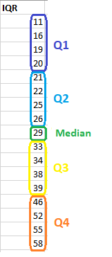
The interquartile range is the middle half of the data. To visualize it, think about the median value that splits the dataset in half. Similarly, you can divide the data into quarters. Statisticians refer to these quarters as quartiles and denote them from low to high as Q1, Q2, Q3, and Q4. The lowest quartile (Q1) contains the quarter of the dataset with the smallest values. The upper quartile (Q4) contains the quarter of the dataset with the highest values. The interquartile range is the middle half of the data that is in between the upper and lower quartiles. In other words, the interquartile range includes the 50% of data points that fall in Q2 and

The IQR is the red area in the graph below.

The interquartile range is a robust measure of variability in a similar manner that the median is a robust measure of central tendency. Neither measure is influenced dramatically by outliers because they don’t depend on every value. Additionally, the interquartile range is excellent for skewed distributions, just like the median. As you’ll learn, when you have a normal distribution, the standard deviation tells you the percentage of observations that fall specific distances from the mean. However, this doesn’t work for skewed distributions, and the IQR is a great alternative.

I’ve divided the dataset below into quartiles. The interquartile range (IQR) extends from the low end of Q2 to the upper limit of Q3. For this dataset, the range is 21 – 39.

Karl Pearson and Rank co-relation

Karl Pearson Coefficient of Correlation (also called the Pearson correlation coefficient or Pearson’s r) is a measure of the strength and direction of the linear relationship between two variables. It ranges from -1 to +1, where +1 indicates a perfect positive linear relationship, -1 indicates a perfect negative linear relationship, and 0 indicates no linear relationship. The formula for Pearson’s r is calculated by dividing the covariance of the two variables by the product of their standard deviations. It is widely used in statistics to analyze the degree of correlation between paired data.

The following are the main properties of correlation.

  1. Coefficient of Correlation lies between -1 and +1:

The coefficient of correlation cannot take value less than -1 or more than one +1. Symbolically,

-1<=r<= + 1 or | r | <1.

  1. Coefficients of Correlation are independent of Change of Origin:

This property reveals that if we subtract any constant from all the values of X and Y, it will not affect the coefficient of correlation.

  1. Coefficients of Correlation possess the property of symmetry:

The degree of relationship between two variables is symmetric as shown below:

  1. Coefficient of Correlation is independent of Change of Scale:

This property reveals that if we divide or multiply all the values of X and Y, it will not affect the coefficient of correlation.

  1. Co-efficient of correlation measures only linear correlation between X and Y.
  2. If two variables X and Y are independent, coefficient of correlation between them will be zero.

Karl Pearson’s Coefficient of Correlation is widely used mathematical method wherein the numerical expression is used to calculate the degree and direction of the relationship between linear related variables.

Pearson’s method, popularly known as a Pearsonian Coefficient of Correlation, is the most extensively used quantitative methods in practice. The coefficient of correlation is denoted by “r”.

If the relationship between two variables X and Y is to be ascertained, then the following formula is used:

Properties of Coefficient of Correlation

  • The value of the coefficient of correlation (r) always lies between±1. Such as:

    r=+1, perfect positive correlation

    r=-1, perfect negative correlation

    r=0, no correlation

  • The coefficient of correlation is independent of the origin and scale.By origin, it means subtracting any non-zero constant from the given value of X and Y the vale of “r” remains unchanged. By scale it means, there is no effect on the value of “r” if the value of X and Y is divided or multiplied by any constant.
  • The coefficient of correlation is a geometric mean of two regression coefficient. Symbolically it is represented as:
  • The coefficient of correlation is “ zero” when the variables X and Y are independent. But, however, the converse is not true.

Assumptions of Karl Pearson’s Coefficient of Correlation

  1. The relationship between the variables is “Linear”, which means when the two variables are plotted, a straight line is formed by the points plotted.
  2. There are a large number of independent causes that affect the variables under study so as to form a Normal Distribution. Such as, variables like price, demand, supply, etc. are affected by such factors that the normal distribution is formed.
  3. The variables are independent of each other.                                     

Note: The coefficient of correlation measures not only the magnitude of correlation but also tells the direction. Such as, r = -0.67, which shows correlation is negative because the sign is “-“ and the magnitude is 0.67.

Spearman Rank Correlation

Spearman rank correlation is a non-parametric test that is used to measure the degree of association between two variables.  The Spearman rank correlation test does not carry any assumptions about the distribution of the data and is the appropriate correlation analysis when the variables are measured on a scale that is at least ordinal.

The Spearman correlation between two variables is equal to the Pearson correlation between the rank values of those two variables; while Pearson’s correlation assesses linear relationships, Spearman’s correlation assesses monotonic relationships (whether linear or not). If there are no repeated data values, a perfect Spearman correlation of +1 or −1 occurs when each of the variables is a perfect monotone function of the other.

Intuitively, the Spearman correlation between two variables will be high when observations have a similar (or identical for a correlation of 1) rank (i.e. relative position label of the observations within the variable: 1st, 2nd, 3rd, etc.) between the two variables, and low when observations have a dissimilar (or fully opposed for a correlation of −1) rank between the two variables.

The following formula is used to calculate the Spearman rank correlation:

ρ = Spearman rank correlation

di = the difference between the ranks of corresponding variables

n = number of observations

Assumptions

The assumptions of the Spearman correlation are that data must be at least ordinal and the scores on one variable must be monotonically related to the other variable.

Data Tabulation

Tabulation is the systematic arrangement of the statistical data in columns or rows. It involves the orderly and systematic presentation of numerical data in a form designed to explain the problem under consideration. Tabulation helps in drawing the inference from the statistical figures.

Tabulation prepares the ground for analysis and interpretation. Therefore a suitable method must be decided carefully taking into account the scope and objects of the investigation, because it is very important part of the statistical methods.

Types of Tabulation

In general, the tabulation is classified in two parts, that is a simple tabulation, and a complex tabulation.

Simple tabulation, gives information regarding one or more independent questions. Complex tabulation gives information regarding two mutually dependent questions.

  • Two-Way Table

These types of table give information regarding two mutually dependent questions. For example, question is, how many millions of the persons are in the Divisions; the One-Way Table will give the answer. But if we want to know that in the population number, who are in the majority, male, or female. The Two-Way Tables will answer the question by giving the column for female and male. Thus the table showing the real picture of divisions sex wise is as under:

  • Three-Way Table

Three-Way Table gives information regarding three mutually dependent and inter-related questions.

For example, from one-way table, we get information about population, and from two-way table, we get information about the number of male and female available in various divisions. Now we can extend the same table to a three way table, by putting a question, “How many male and female are literate?” Thus the collected statistical data will show the following, three mutually dependent and inter-related questions:

  1. Population in various division.
  2. Their sex-wise distribution.
  3. Their position of literacy.

Presentation of Data

Presentation of data is of utter importance nowadays. Afterall everything that’s pleasing to our eyes never fails to grab our attention. Presentation of data refers to an exhibition or putting up data in an attractive and useful manner such that it can be easily interpreted. The three main forms of presentation of data are:

  1. Textual presentation
  2. Data tables
  3. Diagrammatic presentation

Textual Presentation

The discussion about the presentation of data starts off with it’s most raw and vague form which is the textual presentation. In such form of presentation, data is simply mentioned as mere text, that is generally in a paragraph. This is commonly used when the data is not very large.

This kind of representation is useful when we are looking to supplement qualitative statements with some data. For this purpose, the data should not be voluminously represented in tables or diagrams. It just has to be a statement that serves as a fitting evidence to our qualitative evidence and helps the reader to get an idea of the scale of a phenomenon.

For example, “the 2002 earthquake proved to be a mass murderer of humans. As many as 10,000 citizens have been reported dead”. The textual representation of data simply requires some intensive reading. This is because the quantitative statement just serves as an evidence of the qualitative statements and one has to go through the entire text before concluding anything.

Further, if the data under consideration is large then the text matter increases substantially. As a result, the reading process becomes more intensive, time-consuming and cumbersome.

Data Tables or Tabular Presentation

A table facilitates representation of even large amounts of data in an attractive, easy to read and organized manner. The data is organized in rows and columns. This is one of the most widely used forms of presentation of data since data tables are easy to construct and read.

Components of Data Tables

  • Table Number: Each table should have a specific table number for ease of access and locating. This number can be readily mentioned anywhere which serves as a reference and leads us directly to the data mentioned in that particular table.
  • Title: A table must contain a title that clearly tells the readers about the data it contains, time period of study, place of study and the nature of classification of data.
  • Headnotes: A headnote further aids in the purpose of a title and displays more information about the table. Generally, headnotes present the units of data in brackets at the end of a table title.
  • Stubs: These are titles of the rows in a table. Thus a stub display information about the data contained in a particular row.
  • Caption: A caption is the title of a column in the data table. In fact, it is a counterpart if a stub and indicates the information contained in a column.
  • Body or field: The body of a table is the content of a table in its entirety. Each item in a body is known as a ‘cell’.
  • Footnotes: Footnotes are rarely used. In effect, they supplement the title of a table if required.
  • Source: When using data obtained from a secondary source, this source has to be mentioned below the footnote.

Construction of Data Tables

There are many ways for construction of a good table. However, some basic ideas are:

  • The title should be in accordance with the objective of study: The title of a table should provide a quick insight into the table.
  • Comparison: If there might arise a need to compare any two rows or columns then these might be kept close to each other.
  • Alternative location of stubs: If the rows in a data table are lengthy, then the stubs can be placed on the right-hand side of the table.
  • Headings: Headings should be written in a singular form. For example, ‘good’ must be used instead of ‘goods’.
  • Footnote: A footnote should be given only if needed.
  • Size of columns: Size of columns must be uniform and symmetrical.
  • Use of abbreviations: Headings and sub-headings should be free of abbreviations.
  • Units: There should be a clear specification of units above the columns.

Advantages of Tabular Presentation:

  • Ease of representation: A large amount of data can be easily confined in a data table. Evidently, it is the simplest form of data presentation.
  • Ease of analysis: Data tables are frequently used for statistical analysis like calculation of central tendency, dispersion etc.
  • Helps in comparison: In a data table, the rows and columns which are required to be compared can be placed next to each other. To point out, this facilitates comparison as it becomes easy to compare each value.
  • Economical: Construction of a data table is fairly easy and presents the data in a manner which is really easy on the eyes of a reader. Moreover, it saves time as well as space.

Classification of Data and Tabular Presentation

Qualitative Classification

In this classification, data in a table is classified on the basis of qualitative attributes. In other words, if the data contained attributes that cannot be quantified like rural-urban, boys-girls etc. it can be identified as a qualitative classification of data.

Sex Urban Rural
Boys 200 390
Girls 167 100

Quantitative Classification

In quantitative classification, data is classified on basis of quantitative attributes.

Marks No. of Students
0-50 29
51-100 64

Temporal Classification

Here data is classified according to time. Thus when data is mentioned with respect to different time frames, we term such a classification as temporal.

Year Sales
2016 10,000
2017 12,500

Spatial Classification

When data is classified according to a location, it becomes a spatial classification.

Country No. of Teachers
India 139,000
Russia 43,000

Advantages of Tabulation

  1. The large mass of confusing data is easily reduced to reasonable form that is understandable to kind.
  2. The data once arranged in a suitable form, gives the condition of the situation at a glance, or gives a bird eye view.
  3. From the table it is easy to draw some reasonable conclusion or inferences.
  4. Tables gave grounds for analysis of the data.
  5. Errors, and omission if any are always detected in tabulation.

Mean (AM, Weighted, Combined)

Arithmetic Mean

The arithmetic mean,’ mean or average is calculated by summ­ing all the individual observations or items of a sample and divid­ing this sum by the number of items in the sample. For example, as the result of a gas analysis in a respirometer an investigator obtains the following four readings of oxygen percentages:

14.9
10.8
12.3
23.3
Sum = 61.3

He calculates the mean oxygen percentage as the sum of the four items divided by the number of items here, by four. Thus, the average oxygen percentage is

Mean = 61.3 / 4 =15.325%

Calculating a mean presents us with the opportunity for learning statistical symbolism. An individual observation is symbo­lized by Yi, which stands for the ith observation in the sample. Four observations could be written symbolically as Yi, Y2, Y3, Y4.

We shall define n, the sample size, as the number of items in a sample. In this particular instance, the sample size n is 4. Thus, in a large sample, we can symbolize the array from the first to the nth item as follows: Y1, Y2…, Yn. When we wish to sum items, we use the following notation:

The capital Greek sigma, Ʃ, simply means the sum of items indica­ted. The i = 1 means that the items should be summed, starting with the first one, and ending with the nth one as indicated by the i = n above the Ʃ. The subscript and superscript are necessary to indicate how many items should be summed. Below are seen increasing simplifications of the complete notation shown at the extreme left:

Properties of Arithmetic Mean:

  1. The sum of deviations of the items from the arithmetic mean is always zero i.e.

∑(X–X) =0.

  1. The Sum of the squared deviations of the items from A.M. is minimum, which is less than the sum of the squared deviations of the items from any other values.
  2. If each item in the series is replaced by the mean, then the sum of these substitutions will be equal to the sum of the individual items.                       

Merits of A.M:

  1. It is simple to understand and easy to calculate.
  2. It is affected by the value of every item in the series.
  3. It is rigidly defined.
  4. It is capable of further algebraic treatment.
  5. It is calculated value and not based on the position in the series.

Demerits of A.M:

  1. It is affected by extreme items i.e., very small and very large items.
  2. It can hardly be located by inspection.
  3. In some cases A.M. does not represent the actual item. For example, average patients admitted in a hospital is 10.7 per day.
  4. M. is not suitable in extremely asymmetrical distributions.

Weighted Mean

In some cases, you might want a number to have more weight. In that case, you’ll want to find the weighted mean. To find the weighted mean:

  1. Multiply the numbers in your data set by the weights.
  2. Add the results up.

For that set of number above with equal weights (1/5 for each number), the math to find the weighted mean would be:
1(*1/5) + 3(*1/5) + 5(*1/5) + 7(*1/5) + 10(*1/5) = 5.2.

Sample problem: You take three 100-point exams in your statistics class and score 80, 80 and 95. The last exam is much easier than the first two, so your professor has given it less weight. The weights for the three exams are:

  • Exam 1: 40 % of your grade. (Note: 40% as a decimal is .4.)
  • Exam 2: 40 % of your grade.
  • Exam 3: 20 % of your grade.

What is your final weighted average for the class?

  1. Multiply the numbers in your data set by the weights:

    .4(80) = 32

    .4(80) = 32

    .2(95) = 19

  2. Add the numbers up. 32 + 32 + 19 = 83.

The percent weight given to each exam is called a weighting factor.

Weighted Mean Formula

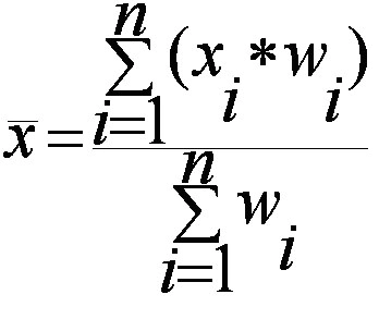
The weighted mean is relatively easy to find. But in some cases the weights might not add up to 1. In those cases, you’ll need to use the weighted mean formula. The only difference between the formula and the steps above is that you divide by the sum of all the weights.

The image above is the technical formula for the weighted mean. In simple terms, the formula can be written as:

Weighted mean = Σwx / Σw

Σ = the sum of (in other words…add them up!).
w = the weights.
x = the value.

To use the formula:

  1. Multiply the numbers in your data set by the weights.
  2. Add the numbers in Step 1 up. Set this number aside for a moment.
  3. Add up all of the weights.
  4. Divide the numbers you found in Step 2 by the number you found in Step 3.

In the sample grades problem above, all of the weights add up to 1 (.4 + .4 + .2) so you would divide your answer (83) by 1:
83 / 1 = 83.

However, let’s say your weighted means added up to 1.2 instead of 1. You’d divide 83 by 1.2 to get:
83 / 1.2 = 69.17.

Combined Mean

A combined mean is a mean of two or more separate groups, and is found by:

  1. Calculating the mean of each group,
  2. Combining the results.

Combined Mean Formula

More formally, a combined mean for two sets can be calculated by the formula :

Where:

  • xa = the mean of the first set,
  • m = the number of items in the first set,
  • xb = the mean of the second set,
  • n = the number of items in the second set,
  • xc the combined mean.

A combined mean is simply a weighted mean, where the weights are the size of each group.

Baye’s Theorem

Bayes’ Theorem is a way to figure out conditional probability. Conditional probability is the probability of an event happening, given that it has some relationship to one or more other events. For example, your probability of getting a parking space is connected to the time of day you park, where you park, and what conventions are going on at any time. Bayes’ theorem is slightly more nuanced. In a nutshell, it gives you the actual probability of an event given information about tests.

“Events” Are different from “tests.” For example, there is a test for liver disease, but that’s separate from the event of actually having liver disease.

Tests are flawed:

Just because you have a positive test does not mean you actually have the disease. Many tests have a high false positive rate. Rare events tend to have higher false positive rates than more common events. We’re not just talking about medical tests here. For example, spam filtering can have high false positive rates. Bayes’ theorem takes the test results and calculates your real probability that the test has identified the event.

Bayes’ Theorem (also known as Bayes’ rule) is a deceptively simple formula used to calculate conditional probability. The Theorem was named after English mathematician Thomas Bayes (1701-1761). The formal definition for the rule is:

In most cases, you can’t just plug numbers into an equation; You have to figure out what your “tests” and “events” are first. For two events, A and B, Bayes’ theorem allows you to figure out p(A|B) (the probability that event A happened, given that test B was positive) from p(B|A) (the probability that test B happened, given that event A happened). It can be a little tricky to wrap your head around as technically you’re working backwards; you may have to switch your tests and events around, which can get confusing. An example should clarify what I mean by “switch the tests and events around.”

Bayes’ Theorem Example

You might be interested in finding out a patient’s probability of having liver disease if they are an alcoholic. “Being an alcoholic” is the test (kind of like a litmus test) for liver disease.

A could mean the event “Patient has liver disease.” Past data tells you that 10% of patients entering your clinic have liver disease. P(A) = 0.10.

B could mean the litmus test that “Patient is an alcoholic.” Five percent of the clinic’s patients are alcoholics. P(B) = 0.05.

You might also know that among those patients diagnosed with liver disease, 7% are alcoholics. This is your B|A: the probability that a patient is alcoholic, given that they have liver disease, is 7%.

Bayes’ theorem tells you:

P(A|B) = (0.07 * 0.1)/0.05 = 0.14

In other words, if the patient is an alcoholic, their chances of having liver disease is 0.14 (14%). This is a large increase from the 10% suggested by past data. But it’s still unlikely that any particular patient has liver disease.

Annuities, Types, Valuation, Uses

An annuity is a financial product that provides certain cash flows at equal time intervals. Annuities are created by financial institutions, primarily life insurance companies, to provide regular income to a client.

An annuity is a reasonable alternative to some other investments as a source of income since it provides guaranteed income to an individual. However, annuities are less liquid than investments in securities because the initially deposited lump sum cannot be withdrawn without penalties.

Upon the issuance of an annuity, an individual pays a lump sum to the issuer of the annuity (financial institution). Then, the issuer holds the amount for a certain period (called an accumulation period). After the accumulation period, the issuer must make fixed payments to the individual according to predetermined time intervals.

Annuities are primarily bought by individuals who want to receive stable retirement income.

Types of Annuities

There are several types of annuities that are classified according to frequency and types of payments. For example, the cash flows of annuities can be paid at different time intervals. The payments can be made weekly, biweekly, or monthly. The primary types of annuities are:

  1. Fixed annuities

Annuities that provide fixed payments. The payments are guaranteed, but the rate of return is usually minimal.

  1. Variable annuities

Annuities that allow an individual to choose a selection of investments that will pay an income based on the performance of the selected investments. Variable annuities do not guarantee the amount of income, but the rate of return is generally higher relative to fixed annuities.

  1. Life annuities

Life annuities provide fixed payments to their holders until his/her death.

  1. Perpetuity

An annuity that provides perpetual cash flows with no end date. Examples of financial instruments that grant the perpetual cash flows to its holders are extremely rare.

The most notable example is a UK Government bond called consol. The first consols were issued in the middle of the 18th century.

Valuation of Annuities

Annuities are valued by discounting the future cash flows of the annuities and finding the present value of the cash flows. The general formula for annuity valuation is:

Uses of Annuities:

  • Retirement Income:

One of the primary uses of annuities is to provide a steady stream of income during retirement. Individuals can convert their retirement savings into an annuity, ensuring they receive regular payments for a specified period or for the rest of their lives. This helps manage longevity risk and provides financial security in retirement.

  • Wealth Management:

Annuities can be used as a wealth management tool, allowing investors to grow their assets on a tax-deferred basis. The accumulation phase of certain annuities lets individuals invest their funds in various financial instruments, potentially increasing their wealth over time before withdrawing it later.

  • Educational Funding:

Parents can use annuities to save for their children’s education. By purchasing an annuity that provides payments when their children reach college age, parents can ensure they have the funds needed to cover tuition and other educational expenses.

  • Structured Settlements:

Annuities are often used in structured settlements resulting from legal claims or personal injury cases. Instead of receiving a lump sum, individuals can opt for an annuity that pays out over time, providing financial stability and reducing the risk of mismanaging a large sum of money.

  • Estate Planning:

Annuities can play a role in estate planning by providing a way to transfer wealth to heirs. Certain types of annuities allow individuals to designate beneficiaries, ensuring that funds are passed on according to their wishes while potentially avoiding probate.

Basic Concepts, Simple and Compound Interest

Interest rates are very powerful and intriguing mathematical concepts. Our banking and finance sector revolves around these interest rates. One minor change in these rates could have tremendous and astonishing impacts over the economy.

Interest is the amount charged by the lender from the borrower on the principal loan sum. It is basically the cost of renting money. And, the rate at which interest is charged on the principal sum is known as the interest rate.

These concepts are categorized into type of interests

  • Simple Interest
  • Compound Interest

Simple Interest

Simple Interest because as the name suggests it is simple and comparatively easy to comprehend.

Simple interest is that type of interest which once credited does not earn interest on itself. It remains fixed over time.

The formula to calculate Simple Interest is

SI = {(P x R x T)/ 100}   

Where,

P = Principal Sum (the original loan/ deposited amount)

R = rate of interest (at which the loan is charged)

T = time period (the duration for which money is borrowed/ deposited)

So, if P amount is borrowed at the rate of interest R for T years then the amount to be repaid to the lender will be

A = P + SI

Compound Interest:

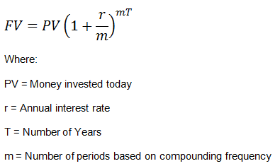
This the most usual type of interest that is used in the banking system and economics. In this kind of interest along with one principal further earns interest on it after the completion of 1-time period. Suppose an amount P is deposited in an account or lent to the borrower that pays compound interest at the rate of R% p.a. Then after n years the deposit or loan will accumulate to:

P ( 1 + R/100)n

Compound Interest when Compounded Half Yearly

Example 2:

Find the compound interest on Rs 8000 for 3/2 years at 10% per annum, interest is payable half-yearly.

Solution: Rate of interest = 10% per annum = 5% per half –year. Time = 3/2 years = 3 half-years

Original principal = Rs 8000.

Amount at the end of the first half-year = Rs 8000 +Rs 400 = Rs 8400

Principal for the second half-year = Rs 8400

Amount at the end of the second half year = Rs 8400 +Rs 420 = Rs 8820

Amount at the end of third half year = Rs 8820 + Rs 441= Rs 9261.

Therefore, compound interest= Rs 9261- Rs 8000 = Rs 1261.

Therefore,

Effective Rate of interest

The Effective Annual Rate (EAR) is the interest rate that is adjusted for compounding over a given period. Simply put, the effective annual interest rate is the rate of interest that an investor can earn (or pay) in a year after taking into consideration compounding.

The Effective Annual Interest Rate is also known as the effective interest rate, effective rate, or the annual equivalent rate. Compare it to the Annual Percentage Rate (APR) which is based on simple interest.

The EAR formula for Effective Annual Interest Rate:

Where:

i = stated annual interest rate

n = number of compounding periods

Importance of Effective Annual Rate

The Effective Annual Interest Rate is an important tool that allows the evaluation of the true return on an investment or true interest rate on a loan.

The stated annual interest rate and the effective interest rate can be significantly different, due to compounding. The effective interest rate is important in figuring out the best loan or determining which investment offers the highest rate of return.

In the case of compounding, the EAR is always higher than the stated annual interest rate.

Relationship between Effective and Nominal rate of interest

Whether effective and nominal rates can ever be the same depends on whether interest calculations involve simple or compound interest. While in a simple interest calculation effective and nominal rates can be the same, effective and nominal rates will never be the same in a compound interest calculation. Although short-term notes generally use simple interest, the majority of interest is calculated using compound interest. To a small-business owner, this means that except when taking out a short-term note, such as loan to fund working capital, effective and nominal rates can be the same for most every other credit purchase or cash investment.

Nominal Vs. Effective Rate

Nominal rates are quoted, published or stated rates for loans, credit cards, savings accounts or other short-term investments. Effective rates are what borrowers or investors actually pay or receive, depending on whether or how frequently interest is compounded. When interest is calculated and added only once, such as in a simple interest calculation, the nominal rate and effective interest rates are equal. With compounding, a calculation in which interest is charged on the loan or investment principal plus any accrued interest up to the point at which interest is being calculated, however, the difference between nominal and effective increases exponentially according to the number of compounding periods. Compounding can take place daily, monthly, quarterly or semi-annually, depending on the account and financial institution regulations.

Simple Interest

The formula for calculating simple interest is “P x I x T” or principle multiplied by the interest rate per period multiplied by the time the money is being borrowed or invested. This formula illustrates that because interest is always being calculated on the principal amount, regardless of the time period involved, the nominal and effective rates will always be equal . If a small-business owner takes out a $5,000 simple interest loan at a nominal rate of 10 percent, $500 of interest will be added to the loan will each year, regardless of the number of years. To illustrate, just as $5,000 x 0.10 x 1 equals $500, $5,000 x 0.10 x 5 equals $2,500 or $500 per year. The nominal and effective rates of 10 percent in both calculations are equal.

Compound Interest

The formula for calculating compound interest shows how nominal and effective rates will never be equal. The formula is “P x (1 + i)n – P” where “n” is the number of compounding periods. In a compound interest calculation, the only time interest is charged or added to the principal is in the first compounding period. The base for each subsequent compounding period is the principal plus any accrued interest. If a small-business owner takes out a one-year $5,000 compound-interest loan at a nominal interest rate of 10 percent, where interest is compounded monthly, total interest that accumulates over the year is $5,000 x (1 + .10)5 – $5,000 or $550. The nominal rate of 10 percent and the effective rate of 11 percent clearly aren’t the same.

Effect On Small Business Owners

It’s crucial that whether the intent is to borrow or invest, small-business owners pay close attention to effective and nominal rates as well as the number of compounding periods. Compounding interest not only creates distance between nominal and effective rates but also works in favor of lenders. For example, a bank, credit card company or auto dealership might advertise a low nominal rate, but compound interest monthly. This in effect significantly increases the total amount owed. This is one reason why lenders advertise or quote nominal rather than effective rates in lending situations.

Relationship between Interest and Discount

The rate charged by the Reserve Bank from the commercial banks and the depository institutions for the overnight loans given to them. The discount rate is fixed by the Federal Reserve Bank and not by the rate of interest in the market.

Also, the discount rate is considered as a rate of interest which is used in the calculation of the present value of the future cash inflows or outflows. The concept of time value of money uses the discount rate to determine the value of certain future cash flows today. Therefore, it is considered important from the investor’s point of view to have a discount rate for the comparison of the value of cash inflows in the future from the cash outflows done to take the given investment.

Interest Rate

If a person called as the lender lends money or some other asset to another person called as the borrower, then the former charges some percentage as interest on the amount given to the later. That percentage is called the interest rate. In financial terms, the rate charged on the principal amount by the bank, financial institutions or other lenders for lending their money to the borrowers is known as the interest rate. It is basically the borrowing cost of using others fund or conversely the amount earned from the lending of funds.

There are two types of interest rate:

  • Simple Interest: In Simple Interest, the interest for every year is charged on the original loan amount only.
  • Compound Interest: In Compound Interest, the interest rate remains same but the sum on which the interest is charged keeps on changing as the interest amount each year is added to the principal amount or the previous year amount for the calculation of interest for the coming year.
error: Content is protected !!