Important Terminologies: Variable, Quantitative Variable, Qualitative Variable, Discrete Variable, Continuous Variable, Dependent Variable, Independent Variable, Frequency, Class Interval, Tally Bar

Important Terminologies:

  • Variable:

Variable is any characteristic, number, or quantity that can be measured or quantified. It can take on different values, which may vary across individuals, objects, or conditions, and is essential in data analysis for observing relationships and patterns.

  • Quantitative Variable:

Quantitative variable is a variable that is measured in numerical terms, such as age, weight, or income. It represents quantities and can be used for mathematical operations, making it suitable for statistical analysis.

  • Qualitative Variable:

Qualitative variable represents categories or attributes, rather than numerical values. Examples include gender, color, or occupation. These variables are non-numeric and are often used in classification and descriptive analysis.

  • Discrete Variable:

Discrete variable is a type of quantitative variable that takes distinct, separate values. These values are countable and cannot take on intermediate values. For example, the number of children in a family is a discrete variable.

  • Continuous Variable:

Continuous variable is a quantitative variable that can take an infinite number of values within a given range. These variables can have decimals or fractions. Examples include height, temperature, or time.

  • Dependent Variable:

Dependent variable is the outcome or response variable that is being measured in an experiment or study. Its value depends on the changes in one or more independent variables. It is the variable of interest in hypothesis testing.

  • Independent Variable:

An independent variable is the variable that is manipulated or controlled in an experiment. It is used to observe its effect on the dependent variable. For example, in a study on plant growth, the amount of water given would be the independent variable.

  • Frequency:

Frequency refers to the number of times a particular value or category occurs in a dataset. It is used in statistical analysis to summarize the distribution of data points within various categories or intervals.

  • Class Interval:

A class interval is a range of values within which data points fall in grouped data. It is commonly used in frequency distributions to organize data into specific ranges, such as “0-10,” “11-20,” etc.

  • Tally Bar:

A tally bar is a method of recording data frequency by using vertical lines. Every group of five tallies (four vertical lines and a fifth diagonal line) represents five occurrences, helping to visually track counts in surveys or experiments.

Important Terminologies in Statistics: Data, Raw Data, Primary Data, Secondary Data, Population, Census, Survey, Sample Survey, Sampling, Parameter, Unit, Variable, Attribute, Frequency, Seriation, Individual, Discrete and Continuous

Statistics is the branch of mathematics that involves the collection, analysis, interpretation, presentation, and organization of data. It helps in drawing conclusions and making decisions based on data patterns, trends, and relationships. Statistics uses various methods such as probability theory, sampling, and hypothesis testing to summarize data and make predictions. It is widely applied across fields like economics, medicine, social sciences, business, and engineering to inform decisions and solve real-world problems.

1. Data

Data is information collected for analysis, interpretation, and decision-making. It can be qualitative (descriptive, such as color or opinions) or quantitative (numerical, such as age or income). Data serves as the foundation for statistical studies, enabling insights into patterns, trends, and relationships.

2. Raw Data

Raw data refers to unprocessed or unorganized information collected from observations or experiments. It is the initial form of data, often messy and requiring cleaning or sorting for meaningful analysis. Examples include survey responses or experimental results.

3. Primary Data

Primary data is original information collected directly by a researcher for a specific purpose. It is firsthand and authentic, obtained through methods like surveys, experiments, or interviews. Primary data ensures accuracy and relevance to the study but can be time-consuming to collect.

4. Secondary Data

Secondary data is pre-collected information used by researchers for analysis. It includes published reports, government statistics, and historical data. Secondary data saves time and resources but may lack relevance or accuracy for specific studies compared to primary data.

5. Population

A population is the entire group of individuals, items, or events that share a common characteristic and are the subject of a study. It includes every possible observation or unit, such as all students in a school or citizens in a country.

6. Census

A census involves collecting data from every individual or unit in a population. It provides comprehensive and accurate information but requires significant resources and time. Examples include national population censuses conducted by governments.

7. Survey

A survey gathers information from respondents using structured tools like questionnaires or interviews. It helps collect opinions, behaviors, or characteristics. Surveys are versatile and widely used in research, marketing, and public policy analysis.

8. Sample Survey

A sample survey collects data from a representative subset of the population. It saves time and costs while providing insights that can generalize to the entire population, provided the sampling method is unbiased and rigorous.

9. Sampling

Sampling is the process of selecting a portion of the population for study. It ensures efficiency and feasibility in data collection. Sampling methods include random, stratified, and cluster sampling, each suited to different study designs.

10. Parameter

A parameter is a measurable characteristic that describes a population, such as the mean, median, or standard deviation. Unlike a statistic, which pertains to a sample, a parameter is specific to the entire population.

11. Unit

A unit is an individual entity in a population or sample being studied. It can represent a person, object, transaction, or observation. Each unit contributes to the dataset, forming the basis for analysis.

12. Variable

A variable is a characteristic or property that can change among individuals or items. It can be quantitative (e.g., age, weight) or qualitative (e.g., color, gender). Variables are the focus of statistical analysis to study relationships and trends.

13. Attribute

An attribute is a qualitative feature that describes a characteristic of a unit. Attributes are non-measurable but observable, such as eye color, marital status, or type of vehicle.

14. Frequency

Frequency represents how often a specific value or category appears in a dataset. It is key in descriptive statistics, helping to summarize and visualize data patterns through tables, histograms, or frequency distributions.

15. Seriation

Seriation is the arrangement of data in sequential or logical order, such as ascending or descending by size, date, or importance. It aids in identifying patterns and organizing datasets for analysis.

16. Individual

An individual is a single member or unit of the population or sample being analyzed. It is the smallest element for data collection and analysis, such as a person in a demographic study or a product in a sales dataset.

17. Discrete Variable

A discrete variable takes specific, separate values, often integers. It is countable and cannot assume fractional values, such as the number of employees in a company or defective items in a batch.

18. Continuous Variable

A continuous variable can take any value within a range and represents measurable quantities. Examples include temperature, height, and time. Continuous variables are essential for analyzing trends and relationships in datasets.

Perquisites of Good Classification of Data

Good classification of data is essential for organizing, analyzing, and interpreting the data effectively. Proper classification helps in understanding the structure and relationships within the data, enabling informed decision-making.

1. Clear Objective

Good classification should have a clear objective, ensuring that the classification scheme serves a specific purpose. It should be aligned with the goal of the study, whether it’s identifying trends, comparing categories, or finding patterns in the data. This helps in determining which variables or categories should be included and how they should be grouped.

2. Homogeneity within Classes

Each class or category within the classification should contain items or data points that are similar to each other. This homogeneity within the classes allows for better analysis and comparison. For example, when classifying people by age, individuals within a particular age group should share certain characteristics related to that age range, ensuring that each class is internally consistent.

3. Heterogeneity between Classes

While homogeneity is crucial within classes, there should be noticeable differences between the various classes. A good classification scheme should maximize the differences between categories, ensuring that each group represents a distinct set of data. This helps in making meaningful distinctions and drawing useful comparisons between groups.

4. Exhaustiveness

Good classification system must be exhaustive, meaning that it should cover all possible data points in the dataset. There should be no omission, and every item must fit into one and only one class. Exhaustiveness ensures that the classification scheme provides a complete understanding of the dataset without leaving any data unclassified.

5. Mutually Exclusive

Classes should be mutually exclusive, meaning that each data point can belong to only one class. This avoids ambiguity and ensures clarity in analysis. For example, if individuals are classified by age group, someone who is 25 years old should only belong to one age class (such as 20-30 years), preventing overlap and confusion.

6. Simplicity

Good classification should be simple and easy to understand. The classification categories should be well-defined and not overly complicated. Simplicity ensures that the classification scheme is accessible and can be easily used for analysis by various stakeholders, from researchers to policymakers. Overly complex classification schemes may lead to confusion and errors.

7. Flexibility

Good classification system should be flexible enough to accommodate new data or changing circumstances. As new categories or data points emerge, the classification scheme should be adaptable without requiring a complete overhaul. Flexibility allows the classification to remain relevant and useful over time, particularly in dynamic fields like business or technology.

8. Consistency

Consistency in classification is essential for maintaining reliability in data analysis. A good classification system ensures that the same criteria are applied uniformly across all classes. For example, if geographical regions are being classified, the same boundaries and criteria should be consistently applied to avoid confusion or inconsistency in reporting.

9. Appropriateness

Good classification should be appropriate for the type of data being analyzed. The classification scheme should fit the nature of the data and the specific objectives of the analysis. Whether classifying data by geographical location, age, or income, the scheme should be meaningful and suited to the research question, ensuring that it provides valuable insights.

Quantitative and Qualitative Classification of Data

Data refers to raw, unprocessed facts and figures that are collected for analysis and interpretation. It can be qualitative (descriptive, like colors or opinions) or quantitative (numerical, like age or sales figures). Data is the foundation of statistics and research, providing the basis for drawing conclusions, making decisions, and discovering patterns or trends. It can come from various sources such as surveys, experiments, or observations. Proper organization and analysis of data are crucial for extracting meaningful insights and informing decisions across various fields.

Quantitative Classification of Data:

Quantitative classification of data involves grouping data based on numerical values or measurable quantities. It is used to organize continuous or discrete data into distinct classes or intervals to facilitate analysis. The data can be categorized using methods such as frequency distributions, where values are grouped into ranges (e.g., 0-10, 11-20) or by specific numerical characteristics like age, income, or height. This classification helps in summarizing large datasets, identifying patterns, and conducting statistical analysis such as finding the mean, median, or mode. It enables clearer insights and easier comparisons of quantitative data across different categories.

Features of Quantitative Classification of Data:

  • Based on Numerical Data

Quantitative classification specifically deals with numerical data, such as measurements, counts, or any variable that can be expressed in numbers. Unlike qualitative data, which deals with categories or attributes, quantitative classification groups data based on values like height, weight, income, or age. This classification method is useful for data that can be measured and involves identifying patterns in numerical values across different ranges.

  • Division into Classes or Intervals

In quantitative classification, data is often grouped into classes or intervals to make analysis easier. These intervals help in summarizing a large set of data and enable quick comparisons. For example, when classifying income levels, data can be grouped into intervals such as “0-10,000,” “10,001-20,000,” etc. The goal is to reduce the complexity of individual data points by organizing them into manageable segments, making it easier to observe trends and patterns.

  • Class Limits

Each class in a quantitative classification has defined class limits, which represent the range of values that belong to that class. For example, in the case of age, a class may be defined with the limits 20-30, where the class includes all data points between 20 and 30 (inclusive). The lower and upper limits are crucial for ensuring that data is classified consistently and correctly into appropriate ranges.

  • Frequency Distribution

Frequency distribution is a key feature of quantitative classification. It refers to how often each class or interval appears in a dataset. By organizing data into classes and counting the number of occurrences in each class, frequency distributions provide insights into the spread of the data. This helps in identifying which ranges or intervals contain the highest concentration of values, allowing for more targeted analysis.

  • Continuous and Discrete Data

Quantitative classification can be applied to both continuous and discrete data. Continuous data, like height or temperature, can take any value within a range and is often classified into intervals. Discrete data, such as the number of people in a group or items sold, involves distinct, countable values. Both types of quantitative data are classified differently, but the underlying principle of grouping into classes remains the same.

  • Use of Central Tendency Measures

Quantitative classification often involves calculating measures of central tendency, such as the mean, median, and mode, for each class or interval. These measures provide insights into the typical or average values within each class. For example, by calculating the average income within specific income brackets, researchers can better understand the distribution of income across the population.

  • Graphical Representation

Quantitative classification is often complemented by graphical tools such as histograms, bar charts, and frequency polygons. These visual representations provide a clear view of how data is distributed across different classes or intervals, making it easier to detect trends, outliers, and patterns. Graphs also help in comparing the frequencies of different intervals, enhancing the understanding of the dataset.

Qualitative Classification of Data:

Qualitative classification of data involves grouping data based on non-numerical characteristics or attributes. This classification is used for categorical data, where the values represent categories or qualities rather than measurable quantities. Examples include classifying individuals by gender, occupation, marital status, or color. The data is typically organized into distinct groups or classes without any inherent order or ranking. Qualitative classification allows researchers to analyze patterns, relationships, and distributions within different categories, making it easier to draw comparisons and identify trends. It is often used in fields such as social sciences, marketing, and psychology for descriptive analysis.

Features of  Qualitative Classification of Data:

  • Based on Categories or Attributes

Qualitative classification deals with data that is based on categories or attributes, such as gender, occupation, religion, or color. Unlike quantitative data, which is measured in numerical values, qualitative data involves sorting or grouping items into distinct categories based on shared qualities or characteristics. This type of classification is essential for analyzing data that does not have a numerical relationship.

  • No Specific Order or Ranking

In qualitative classification, the categories do not have a specific order or ranking. For instance, when classifying individuals by their profession (e.g., teacher, doctor, engineer), the categories do not imply any hierarchy or ranking order. The lack of a natural sequence or order distinguishes qualitative classification from ordinal data, which involves categories with inherent ranking (e.g., low, medium, high). The focus is on grouping items based on their similarity in attributes.

  • Mutual Exclusivity

Each data point in qualitative classification must belong to one and only one category, ensuring mutual exclusivity. For example, an individual cannot simultaneously belong to both “Male” and “Female” categories in a gender classification scheme. This feature helps to avoid overlap and ambiguity in the classification process. Ensuring mutual exclusivity is crucial for clear analysis and accurate data interpretation.

  • Exhaustiveness

Qualitative classification should be exhaustive, meaning that all possible categories are covered. Every data point should fit into one of the predefined categories. For instance, if classifying by marital status, categories like “Single,” “Married,” “Divorced,” and “Widowed” must encompass all possible marital statuses within the dataset. Exhaustiveness ensures no data is left unclassified, making the analysis complete and comprehensive.

  • Simplicity and Clarity

A good qualitative classification should be simple, clear, and easy to understand. The categories should be well-defined, and the criteria for grouping data should be straightforward. Complexity and ambiguity in categorization can lead to confusion, misinterpretation, or errors in analysis. Simple and clear classification schemes make the data more accessible and improve the quality of research and reporting.

  • Flexibility

Qualitative classification is flexible and can be adapted as new categories or attributes emerge. For example, in a study of professions, new job titles or fields may develop over time, and the classification system can be updated to include these new categories. Flexibility in qualitative classification allows researchers to keep the data relevant and reflective of changes in society, industry, or other fields of interest.

  • Focus on Descriptive Analysis

Qualitative classification primarily focuses on descriptive analysis, which involves summarizing and organizing data into meaningful categories. It is used to explore patterns and relationships within the data, often through qualitative techniques such as thematic analysis or content analysis. The goal is to gain insights into the characteristics or behaviors of individuals, groups, or phenomena rather than making quantitative comparisons.

Calculation of Interest

Calculating interest rate is not at all a difficult method to understand. Knowing to calculate interest rate can solve a lot of wages problems and save money while taking investment decisions. There is an easy formula to calculate simple interest rates. If you are aware of your loan and interest amount you can pay, you can do the largest interest rate calculation for yourself.

Using the simple interest calculation formula, you can also see your interest payments in a year and calculate your annual percentage rate.

Here is the step by step guide to calculate the interest rate.

How to calculate interest rate?

Know the formula which can help you to calculate your interest rate.

Step 1

To calculate your interest rate, you need to know the interest formula I/Pt = r to get your rate. Here,

I = Interest amount paid in a specific time period (month, year etc.)

P = Principle amount (the money before interest)

t = Time period involved

r = Interest rate in decimal

You should remember this equation to calculate your basic interest rate.

Step 2

Once you put all the values required to calculate your interest rate, you will get your interest rate in decimal. Now, you need to convert the interest rate you got by multiplying it by 100. For example, a decimal like .11 will not help much while figuring out your interest rate. So, if you want to find your interest rate for .11, you have to multiply .11 with 100 (.11 x 100).

For this case, your interest rate will be (.11 x 100 = 11) 11%.

Step 3

Apart from this, you can also calculate your time period involved, principal amount and interest amount paid in a specific time period if you have other inputs available with you.

Calculate interest amount paid in a specific time period, I = Prt.

Calculate the principal amount, P = I/rt.

Calculate time period involved t = I/Pr.

Step 4

Most importantly, you have to make sure that your time period and interest rate are following the same parameter.

For example, on a loan, you want to find your monthly interest rate after one year. In this case, if you put t = 1, you will get the final interest rate as the interest rate per year. Whereas, if you want the monthly interest rate, you have to put the correct amount of time elapsed. Here, you can consider the time period like 12 months.

Please remember, your time period should be the same time amount as the interest paid. For example, if you’re calculating a year’s monthly interest payments then, it can be considered you’ve made 12 payments.

Also, you have to make sure that you check the time period (weekly, monthly, yearly etc.) when your interest is calculated with your bank.

Step 5

You can rely on online calculators to get interest rates for complex loans, such as mortgages. You should also know the interest rate of your loan when you sign up for it.

For fluctuating rates, sometimes it becomes difficult to determine what a certain rate means. So, it is better to use free online calculators by searching “variable APR interest calculator”, “mortgage interest calculator” etc.

Calculation of interest when rate of interest and cash price is given

  • Where Cash Price, Interest Rate and Instalment are Given:

Illustration:

On 1st January 2003, A bought a television from a seller under Hire Purchase System, the cash price of which being Rs 10.450 as per the following terms:

(a) Rs 3,000 to be paid on signing the agreement.

(b) Balance to be paid in three equal installments of Rs 3,000 at the end of each year,

(c) The rate of interest charged by the seller is 10% per annum.

You are required to calculate the interest paid by the buyer to the seller each year.

Solution:

Note:

  1. there is no time gap between the signing of the agreement and the cash down payment of Rs 3,000 (1.1.2003). Hence no interest is calculated. The entire amount goes to reduce the cash price.
  2. The interest in the last installment is taken at the differential figure of Rs 285.50 (3,000 – 2,714.50).

(2) Where Cash Price and Installments are Given but Rate of Interest is Omitted:

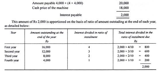
Where the rate of interest is not given and only the cash price and the total payments under hire purchase installments are given, then the total interest paid is the difference between the cash price of the asset and the total amount paid as per the agreement. This interest amount is apportioned in the ratio of amount outstanding at the end of each period.

Illustration:

Mr. A bought a machine under hire purchase agreement, the cash price of the machine being Rs 18,000. As per the terms, the buyer has to pay Rs 4,000 on signing the agreement and the balance in four installments of Rs 4,000 each, payable at the end of each year. Calculate the interest chargeable at the end of each year.

(3) Where installments and Rate of Interest are Given but Cash Value of the Asset is Omitted:

In certain problems, the cash price is not given. It is necessary that we must first find out the cash price and interest included in the installments. The asset account is to be debited with the actual price of the asset. Under such situations, i.e. in the absence of cash price, the interest is calculated from the last year.

It may be noted that the amount of interest goes on increasing from 3rd year to 2nd year, 2nd year to 1st year. Since the interest is included in the installments and by knowing the rate of interest, we can find out the cash price.

Thus:

Let the cash price outstanding be: Rs 100

Interest @ 10% on Rs 100 for a year: Rs 10

Installment paid at the end of the year 110

The interest on installment price = 10/110 or 1/11 as a ratio.

Illustration:

I buy a television on Hire Purchase System.

The terms of payment are as follows:

Rs 2,000 to be paid on signing the agreement;

Rs 2,800 at the end of the first year;

Rs 2,600 at the end of the second year;

Rs 2,400 at the end of the third year;

Rs 2,200 at the end of the fourth year.

If interest is charged at the rate of 10% p.a., what was the cash value of the television?

Solution:

(4) Calculation of Cash Price when Reference to Annuity Table, the Rate of Interest and Installments are Given:

Sometimes in the problem a reference to annuity table wherein present value of the annuity for a number of years at a certain rate of interest is given. In such cases the cash price is calculated by multiplying the amount of installment and adding the product to the initial payment.

Illustration:

A agrees to purchase a machine from a seller under Hire Purchase System by annual installment of Rs 10,000 over a period of 5 years. The seller charges interest at 4% p.a. on yearly balance.

N.B. The present value of Re 1 p.a. for five years at 4% is Rs 4.4518. Find out the cash price of the machine.

Solution:

Installment Re 1 Present value = Rs 4.4518

Installment = Rs 10,000 Present value = Rs 4.4518 x 10,000 = Rs 44,518

Credit: https://www.yourarticlelibrary.com/accounting/hire-purchase/how-to-calculate-interest-4-cases-hire-purchase/51175

Quantitative Methods for Business – 1

Unit 1 Number System {Book}

Natural Numbers, Even Numbers, Odd Numbers

VIEW

Integers, Prime Numbers

VIEW

Rational & Irrational numbers

VIEW

Real Numbers, HCF & LCM (Simple Problems)

VIEW

Unit 2 Theory Of Equations {Book}

Please refer Books for this Unit

VIEW

Unit 3 Progressions {Book}

Arithmetic Progression Finding the “n”th term of AP and Sum to “n”th term of AP.

VIEW

Insertion of Arithmetic Mean

VIEW

Geometric Progression Finding the “n”th term of GP and

VIEW

Insertion of Geometric Mean

VIEW

Unit 4 Matrices and Determinants {Book}

Please refer Books for this Unit

VIEW

Unit 4 Commercial Arithmetic {Book}

Simple Interest, Compound Interest including half yearly and quarterly calculations

VIEW

Annuities

VIEW

Percentages

VIEW

Bills Discounting

VIEW

Ratios and proportions

VIEW

Duplicate: Triplicate and Sub-duplicate of a ratio

VIEW

Proportions: Third, Fourth and inverse proportion

VIEW

Unit 5 Progressions {Book}

Arithmetic Progression Finding the “n”th term of AP and Sum to “n”th term of AP.

VIEW

Insertion of Arithmetic Mean

VIEW

Geometric Progression Finding the “n”th term of GP and

VIEW

Insertion of Geometric Mean

VIEW

Determinants of the Value of Bonds

Bonds are fixed-income securities that represent a loan from an investor to a borrower, typically a corporation or government. When purchasing a bond, the investor lends money in exchange for periodic interest payments and the return of the bond’s face value at maturity. Bonds are used to finance various projects and operations, providing a predictable income stream for investors.

Valuation of Bonds

The method for valuation of bonds involves three steps as follows:

Step 1: Estimate the expected cash flows

Step 2: Determine the appropriate interest rate that should be used to discount the cash flows.

& Step 3: Calculate the present value of the expected cash flows (step-1) using appropriate interest rate (step- 2) i.e. discounting the expected cash flows

Step 1: Estimating cash flows

Cash flow is the cash that is estimated to be received in future from investment in a bond. There are only two types of cash flows that can be received from investment in bonds i.e. coupon payments and principal payment at maturity.

The usual cash flow cycle of the bond is coupon payments are received at regular intervals as per the bond agreement, and final coupon plus principle payment is received at the maturity. There are some instances when bonds don’t follow these regular patterns. Unusual patterns maybe a result of the different type of bond such as zero-coupon bonds, in which there are no coupon payments. Considering such factors, it is important for an analyst to estimate accurate cash flow for the purpose of bond valuation.

Step 2: Determine the appropriate interest rate to discount the cash flows

Once the cash flow for the bond is estimated, the next step is to determine the appropriate interest rate to discount cash flows. The minimum interest rate that an investor should require is the interest available in the marketplace for default-free cash flow. Default-free cash flows are cash flows from debt security which are completely safe and has zero chances default. Such securities are usually issued by the central bank of a country, for example, in the USA it is bonds by U.S. Treasury Security.

Consider a situation where an investor wants to invest in bonds. If he is considering to invest corporate bonds, he is expecting to earn higher return from these corporate bonds compared to rate of returns of U.S. Treasury Security bonds. This is because chances are that a corporate bond might default, whereas the U.S. Security Treasury bond is never going to default. As he is taking a higher risk by investing in corporate bonds, he expects a higher return.

One may use single interest rate or multiple interest rates for valuation.

Step 3: Discounting the expected cash flows

Now that we already have values of expected future cash flows and interest rate used to discount the cash flow, it is time to find the present value of cash flows. Present Value of a cash flow is the amount of money that must be invested today to generate a specific future value. The present value of a cash flow is more commonly known as discounted value.

The present value of a cash flow depends on two determinants:

  • When a cash flow will be received i.e. timing of a cash flow &;
  • The required interest rate, more widely known as Discount Rate (rate as per Step-2)

First, we calculate the present value of each expected cash flow. Then we add all the individual present values and the resultant sum is the value of the bond.

The formula to find the present value of one cash flow is:

Present value formula for Bond Valuation

Present Value n = Expected cash flow in the period n/ (1+i) n

Here,

i = rate of return/discount rate on bond
n = expected time to receive the cash flow

By this formula, we will get the present value of each individual cash flow t years from now. The next step is to add all individual cash flows.

Bond Value = Present Value 1 + Present Value 2 + ……. + Present Value n

Sampling and Sampling Distribution

Sample design is the framework, or road map, that serves as the basis for the selection of a survey sample and affects many other important aspects of a survey as well. In a broad context, survey researchers are interested in obtaining some type of information through a survey for some population, or universe, of interest. One must define a sampling frame that represents the population of interest, from which a sample is to be drawn. The sampling frame may be identical to the population, or it may be only part of it and is therefore subject to some under coverage, or it may have an indirect relationship to the population.

Sampling is the process of selecting a subset of individuals, items, or observations from a larger population to analyze and draw conclusions about the entire group. It is essential in statistics when studying the entire population is impractical, time-consuming, or costly. Sampling can be done using various methods, such as random, stratified, cluster, or systematic sampling. The main objectives of sampling are to ensure representativeness, reduce costs, and provide timely insights. Proper sampling techniques enhance the reliability and validity of statistical analysis and decision-making processes.

Steps in Sample Design

While developing a sampling design, the researcher must pay attention to the following points:

  • Type of Universe:

The first step in developing any sample design is to clearly define the set of objects, technically called the Universe, to be studied. The universe can be finite or infinite. In finite universe the number of items is certain, but in case of an infinite universe the number of items is infinite, i.e., we cannot have any idea about the total number of items. The population of a city, the number of workers in a factory and the like are examples of finite universes, whereas the number of stars in the sky, listeners of a specific radio programme, throwing of a dice etc. are examples of infinite universes.

  • Sampling unit:

A decision has to be taken concerning a sampling unit before selecting sample. Sampling unit may be a geographical one such as state, district, village, etc., or a construction unit such as house, flat, etc., or it may be a social unit such as family, club, school, etc., or it may be an individual. The researcher will have to decide one or more of such units that he has to select for his study.

  • Source list:

It is also known as ‘sampling frame’ from which sample is to be drawn. It contains the names of all items of a universe (in case of finite universe only). If source list is not available, researcher has to prepare it. Such a list should be comprehensive, correct, reliable and appropriate. It is extremely important for the source list to be as representative of the population as possible.

  • Size of Sample:

This refers to the number of items to be selected from the universe to constitute a sample. This a major problem before a researcher. The size of sample should neither be excessively large, nor too small. It should be optimum. An optimum sample is one which fulfills the requirements of efficiency, representativeness, reliability and flexibility. While deciding the size of sample, researcher must determine the desired precision as also an acceptable confidence level for the estimate. The size of population variance needs to be considered as in case of larger variance usually a bigger sample is needed. The size of population must be kept in view for this also limits the sample size. The parameters of interest in a research study must be kept in view, while deciding the size of the sample. Costs too dictate the size of sample that we can draw. As such, budgetary constraint must invariably be taken into consideration when we decide the sample size.

  • Parameters of interest:

In determining the sample design, one must consider the question of the specific population parameters which are of interest. For instance, we may be interested in estimating the proportion of persons with some characteristic in the population, or we may be interested in knowing some average or the other measure concerning the population. There may also be important sub-groups in the population about whom we would like to make estimates. All this has a strong impact upon the sample design we would accept.

  • Budgetary constraint:

Cost considerations, from practical point of view, have a major impact upon decisions relating to not only the size of the sample but also to the type of sample. This fact can even lead to the use of a non-probability sample.

  • Sampling procedure:

Finally, the researcher must decide the type of sample he will use i.e., he must decide about the technique to be used in selecting the items for the sample. In fact, this technique or procedure stands for the sample design itself. There are several sample designs (explained in the pages that follow) out of which the researcher must choose one for his study. Obviously, he must select that design which, for a given sample size and for a given cost, has a smaller sampling error.

Types of Samples

  • Probability Sampling (Representative samples)

Probability samples are selected in such a way as to be representative of the population. They provide the most valid or credible results because they reflect the characteristics of the population from which they are selected (e.g., residents of a particular community, students at an elementary school, etc.). There are two types of probability samples: random and stratified.

  • Random Sample

The term random has a very precise meaning. Each individual in the population of interest has an equal likelihood of selection. This is a very strict meaning you can’t just collect responses on the street and have a random sample.

The assumption of an equal chance of selection means that sources such as a telephone book or voter registration lists are not adequate for providing a random sample of a community. In both these cases there will be a number of residents whose names are not listed. Telephone surveys get around this problem by random-digit dialling but that assumes that everyone in the population has a telephone. The key to random selection is that there is no bias involved in the selection of the sample. Any variation between the sample characteristics and the population characteristics is only a matter of chance.

  • Stratified Sample

A stratified sample is a mini-reproduction of the population. Before sampling, the population is divided into characteristics of importance for the research. For example, by gender, social class, education level, religion, etc. Then the population is randomly sampled within each category or stratum. If 38% of the population is college-educated, then 38% of the sample is randomly selected from the college-educated population.

Stratified samples are as good as or better than random samples, but they require fairly detailed advance knowledge of the population characteristics, and therefore are more difficult to construct.

  • Non-probability Samples (Non-representative samples)

As they are not truly representative, non-probability samples are less desirable than probability samples. However, a researcher may not be able to obtain a random or stratified sample, or it may be too expensive. A researcher may not care about generalizing to a larger population. The validity of non-probability samples can be increased by trying to approximate random selection, and by eliminating as many sources of bias as possible.

  • Quota Sample

The defining characteristic of a quota sample is that the researcher deliberately sets the proportions of levels or strata within the sample. This is generally done to insure the inclusion of a particular segment of the population. The proportions may or may not differ dramatically from the actual proportion in the population. The researcher sets a quota, independent of population characteristics.

Example: A researcher is interested in the attitudes of members of different religions towards the death penalty. In Iowa a random sample might miss Muslims (because there are not many in that state). To be sure of their inclusion, a researcher could set a quota of 3% Muslim for the sample. However, the sample will no longer be representative of the actual proportions in the population. This may limit generalizing to the state population. But the quota will guarantee that the views of Muslims are represented in the survey.

  • Purposive Sample

A purposive sample is a non-representative subset of some larger population, and is constructed to serve a very specific need or purpose. A researcher may have a specific group in mind, such as high level business executives. It may not be possible to specify the population they would not all be known, and access will be difficult. The researcher will attempt to zero in on the target group, interviewing whoever is available.

  • Convenience Sample

A convenience sample is a matter of taking what you can get. It is an accidental sample. Although selection may be unguided, it probably is not random, using the correct definition of everyone in the population having an equal chance of being selected. Volunteers would constitute a convenience sample.

Non-probability samples are limited with regard to generalization. Because they do not truly represent a population, we cannot make valid inferences about the larger group from which they are drawn. Validity can be increased by approximating random selection as much as possible, and making every attempt to avoid introducing bias into sample selection.

Sampling Distribution

Sampling Distribution is a statistical concept that describes the probability distribution of a given statistic (e.g., mean, variance, or proportion) derived from repeated random samples of a specific size taken from a population. It plays a crucial role in inferential statistics, providing the foundation for making predictions and drawing conclusions about a population based on sample data.

Concepts of Sampling Distribution

A sampling distribution is the distribution of a statistic (not raw data) over all possible samples of the same size from a population. Commonly used statistics include the sample mean (Xˉ\bar{X}), sample variance, and sample proportion.

Purpose:

It allows statisticians to estimate population parameters, test hypotheses, and calculate probabilities for statistical inference.

Shape and Characteristics:

    • The shape of the sampling distribution depends on the population distribution and the sample size.
    • For large sample sizes, the Central Limit Theorem states that the sampling distribution of the mean will be approximately normal, regardless of the population’s distribution.

Importance of Sampling Distribution

  • Facilitates Statistical Inference:

Sampling distributions are used to construct confidence intervals and perform hypothesis tests, helping to infer population characteristics.

  • Standard Error:

The standard deviation of the sampling distribution, called the standard error, quantifies the variability of the sample statistic. Smaller standard errors indicate more reliable estimates.

  • Links Population and Samples:

It provides a theoretical framework that connects sample statistics to population parameters.

Types of Sampling Distributions

  • Distribution of Sample Means:

Shows the distribution of means from all possible samples of a population.

  • Distribution of Sample Proportions:

Represents the proportion of a certain outcome in samples, used in binomial settings.

  • Distribution of Sample Variances:

Explains the variability in sample data.

Example

Consider a population of students’ test scores with a mean of 70 and a standard deviation of 10. If we repeatedly draw random samples of size 30 and calculate the sample mean, the distribution of those means forms the sampling distribution. This distribution will have a mean close to 70 and a reduced standard deviation (standard error).

Present Value, Functions

Present Value (PV) concept refers to the current worth of a future sum of money or stream of cash flows, discounted at a specific interest rate. It reflects the principle that a dollar today is worth more than a dollar in the future due to its potential earning capacity.

PV = FV / (1+r)^n

where

FV is the future value,

r is the discount rate,

n is the number of periods until payment.

This concept is essential in finance for assessing investment opportunities and financial planning.

Functions of Present Value:

  • Valuation of Cash Flows:

PV allows investors and analysts to evaluate the worth of future cash flows generated by an investment. By discounting future cash flows to their present value, stakeholders can determine if the investment is financially viable compared to its cost.

  • Investment Decision Making:

In capital budgeting, PV is crucial for assessing whether to proceed with projects or investments. By comparing the present value of expected cash inflows to the initial investment (cost), decision-makers can prioritize projects that offer the highest returns relative to their costs.

  • Comparison of Investment Alternatives:

PV provides a standardized method for comparing different investment opportunities. By converting future cash flows into their present values, investors can effectively evaluate and contrast various investments, regardless of their cash flow patterns or timing.

  • Financial Planning:

Individuals and businesses use PV for financial planning and retirement savings. By calculating the present value of future financial goals (like retirement funds), individuals can determine how much they need to save and invest today to achieve those goals.

  • Debt Valuation:

PV is essential for valuing bonds and other debt instruments. The present value of future interest payments and the principal repayment is calculated to determine the fair market value of the bond. This valuation helps investors make informed decisions about purchasing or selling bonds.

  • Risk Assessment:

Present Value helps in assessing the risk associated with investments. Higher discount rates, which account for risk and uncertainty, lower the present value of future cash flows. This relationship allows investors to gauge the risk-return trade-off of different investments effectively.

Future Value, Functions

Future Value (FV) is the value of a current asset at a future date based on an assumed rate of growth. The future value (FV) is important to investors and financial planners as they use it to estimate how much an investment made today will be worth in the future. Knowing the future value enables investors to make sound investment decisions based on their anticipated needs.

FV calculation allows investors to predict, with varying degrees of accuracy, the amount of profit that can be generated by different investments. The amount of growth generated by holding a given amount in cash will likely be different than if that same amount were invested in stocks; so, the FV equation is used to compare multiple options.

Determining the FV of an asset can become complicated, depending on the type of asset. Also, the FV calculation is based on the assumption of a stable growth rate. If money is placed in a savings account with a guaranteed interest rate, then the FV is easy to determine accurately. However, investments in the stock market or other securities with a more volatile rate of return can present greater difficulty.

Future Value (FV) formula assumes a constant rate of growth and a single upfront payment left untouched for the duration of the investment. The FV calculation can be done one of two ways depending on the type of interest being earned. If an investment earns simple interest, then the Future Value (FV) formula is:

  • Future value (FV) is the value of a current asset at some point in the future based on an assumed growth rate.
  • Investors are able to reasonably assume an investment’s profit using the future value (FV) calculation.
  • Determining the future value (FV) of a market investment can be challenging because of the market’s volatility.
  • There are two ways of calculating the future value (FV) of an asset: FV using simple interest and FV using compound interest.

Functions of Future Value:

  • Investment Growth Measurement:

FV is used to calculate how much an investment will grow over time. By applying a specified interest rate, investors can estimate the future worth of their initial investments or savings, helping them understand the potential returns.

  • Retirement Planning:

FV plays a critical role in retirement planning. Individuals can determine how much they need to save today to achieve a desired retirement income. By calculating the future value of regular contributions to retirement accounts, they can set realistic savings goals.

  • Loan Repayment Calculations:

For borrowers, FV is crucial in understanding the total amount owed on loans over time. It helps them visualize the long-term cost of borrowing, including interest payments, aiding in budgeting and financial decision-making.

  • Comparison of Investment Opportunities:

FV provides a standardized way to compare different investment options. By calculating the future value of various investment opportunities, investors can evaluate which options offer the highest potential returns over a specified period.

  • Education Funding:

Parents can use FV to plan for their children’s education expenses. By estimating future tuition costs and calculating how much they need to save now, parents can ensure they accumulate sufficient funds by the time their children enter college.

  • Inflation Adjustment:

FV helps investors account for inflation when planning for future expenses. By incorporating an expected inflation rate into future value calculations, individuals and businesses can better estimate the amount needed to maintain purchasing power over time.

error: Content is protected !!