Tag: Market Power

Business decisions are pivotal for the success of an organization, and they are often made in response to various economic problems. These problems can arise from both internal factors (like management inefficiencies or resource allocation issues) and external factors (like market competition or changes in government policies). Effective business decisions are a blend of understanding economic principles, analyzing data, and predicting future trends.

Nature of Economic Problems

Economic problems arise due to the basic issue of scarcity. Resources are limited, but human wants are infinite. This leads to three fundamental economic problems that businesses face:

• What to produce?:

Businesses must decide what goods and services to produce. Given limited resources, it’s crucial to identify which products will generate the most value for the business while meeting customer demands. Misjudging this can lead to a misallocation of resources and financial losses.

• How to produce?:

This pertains to the methods and techniques used in the production process. A business must choose the most efficient combination of labor, capital, and technology. The decision on how to produce is influenced by factors like cost efficiency, technological advancements, and labor availability.

• For whom to produce?:

This relates to identifying the target market and determining how to allocate the produced goods or services. The distribution of goods depends on the purchasing power of different segments of the population, and businesses must decide how to maximize profits while catering to diverse consumer groups.

These fundamental problems require businesses to make constant decisions regarding resource allocation, production techniques, and market segmentation.

Economic Problems Impacting Business Decisions

• Resource Scarcity:

One of the primary economic problems that businesses face is scarcity. With limited resources available, businesses must prioritize their production and investment decisions. Scarcity forces firms to make choices about which products to produce, how to allocate capital, and how to manage labor.

• Inflation:

Inflation, or the rise in prices over time, affects the purchasing power of consumers and the cost of production. In an inflationary environment, businesses may face increased costs for raw materials, labor, and utilities. To manage this, companies need to adjust pricing strategies, cut costs, or innovate to maintain profitability.

• Uncertainty:

Uncertainty in the economy, such as fluctuations in demand, technological changes, or political instability, can disrupt business decisions. Businesses must forecast potential outcomes and adopt risk management strategies to navigate these uncertainties. This often leads to decisions like diversifying product lines or entering new markets to reduce dependence on a single revenue stream.

• Market Competition:

Competition in the market also presents an economic challenge. The presence of numerous firms offering similar goods and services forces businesses to be more strategic in their pricing, marketing, and production decisions. Understanding the nature of market competition helps a business decide whether to focus on cost leadership, differentiation, or innovation.

Types of Business Decisions

• Strategic Decisions:

These are long-term decisions that define the direction of the business. Examples include entering new markets, investing in new technologies, or changing business models. Strategic decisions are heavily influenced by economic problems like market trends, resource availability, and technological advancements.

• Tactical Decisions:

These are medium-term decisions that aim to implement the strategies laid out by the business. These may involve decisions on production methods, inventory management, or pricing strategies. Economic problems such as inflation or changes in consumer preferences often drive these decisions.

• Operational Decisions:

These are short-term decisions concerned with day-to-day operations. They are aimed at improving efficiency and reducing costs. Examples include managing employee shifts, setting daily production targets, or adjusting prices based on competitor actions. Operational decisions are highly responsive to economic problems like changes in labor costs or supply chain disruptions.

Economic Theories for Decision-Making

• Microeconomics:

Businesses use microeconomic principles to assess how individuals and firms make choices about the allocation of resources. These principles help in setting prices, determining output levels, and deciding on the most cost-effective production methods.

• Cost-Benefit Analysis:

This involves comparing the costs of a decision with the expected benefits. The goal is to determine whether the benefits of a decision outweigh the costs, guiding businesses toward more profitable choices.

• Market Structures:

Understanding different market structures (perfect competition, monopolistic competition, oligopoly, and monopoly) helps businesses decide on pricing strategies, production levels, and marketing approaches.

The Law of equimarginal Utility is another fundamental principle of Econo­mics. This law is also known as the Law of substitution or the Law of Maxi­mum Satisfaction.

We know that human wants are unlimited whereas the means to satisfy these wants are strictly limited. It, therefore’ becomes necessary to pick up the most urgent wants that can be satisfied with the money that a consumer has. Of the things that he decides to buy he must buy just the right quantity. Every prudent consumer will try to make the best use of the money at his disposal and derive the maximum satisfaction.

Explanation of the Law

In order to get maximum satisfaction out of the funds we have, we carefully weigh the satisfaction obtained from each rupee ‘had we spend If we find that a rupee spent in one direction has greater utility than in another, we shall go on spending money on the former commodity, till the satisfaction derived from the last rupee spent in the two cases is equal.

It other words, we substitute some units of the commodity of greater utility tor some units of the commodity of less utility. The result of this substitution will be that the marginal utility of the former will fall and that of the latter will rise, till the two marginal utilities are equalized. That is why the law is also called the Law of Substitution or the Law of equimarginal Utility.

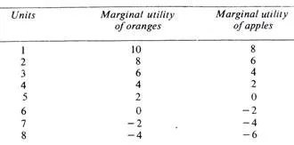
Suppose apples and oranges are the two commodities to be purchased. Suppose further that we have got seven rupees to spend. Let us spend three rupees on oranges and four rupees on apples. What is the result? The utility of the 3rd unit of oranges is 6 and that of the 4th unit of apples is 2. As the marginal utility of oranges is higher, we should buy more of oranges and less of apples. Let us substitute one orange for one apple so that we buy four oranges and three apples.

Now the marginal utility of both oranges and apples is the same, i.e., 4. This arrangement yields maximum satisfaction. The total utility of 4 oranges would be 10 + 8 + 6 + 4 = 28 and of three apples 8 + 6 + 4= 18 which gives us a total utility of 46. The satisfaction given by 4 oranges and 3 apples at one rupee each is greater than could be obtained by any other combination of apples and oranges. In no other case does this utility amount to 46. We may take some other combinations and see.

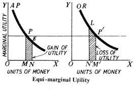
We thus come to the conclusion that we obtain maximum satisfaction when we equalize marginal utilities by substituting some units of the more useful for the less useful commodity. We can illustrate this principle with the help of a diagram.

Diagrammatic Representation:

In the two figures given below, OX and OY are the two axes. On X-axis OX are represented the units of money and on the Y-axis marginal utilities. Suppose a person has 7 rupees to spend on apples and oranges whose diminishing marginal utilities are shown by the two curves AP and OR respectively.

The consumer will gain maximum satisfaction if he spends OM money (3 rupees) on apples and OM’ money (4 rupees) on oranges because in this situation the marginal utilities of the two are equal (PM = P’M’). Any other combination will give less total satisfaction.

Let the purchase spend MN money (one rupee) more on apples and the same amount of money, N’M’(= MN) less on oranges. The diagram shows a loss of utility represented by the shaded area LN’M’P’ and a gain of PMNE utility. As MN = N’M’ and PM=P’M’, it is proved that the area LN’M’P’ (loss of utility from reduced consumption of oranges) is bigger than PMNE (gain of utility from increased consumption of apples). Hence the total utility of this new combination is less.

We then, conclude that no other combination of apples and oranges gives as great a satisfaction to the consumer as when PM = P’M’, i.e., where the marginal utilities of apples and oranges purchased are equal, with given amour, of money at our disposal.

Limitations of the Law of Equimarginal Utility

Like other economic laws, the law of equimarginal utility too has certain limitations or exceptions. The following are the main exception.

(i) Ignorance

If the consumer is ignorant or blindly follows custom or fashion, he will make a wrong use of money. On account of his ignorance he may not know where the utility is greater and where less. Thus, ignorance may prevent him from making a rational use of money. Hence, his satisfaction may not be the maximum, because the marginal utilities from his expenditure can­not be equalised due to ignorance.

(ii) Inefficient Organisation

In the same manner, an incompetent organ­iser of business will fail to achieve the best results from the units of land, labour and capital that he employs. This is so because he may not be able to divert expenditure to more profitable channels from the less profitable ones.

(iii) Unlimited Resources

The law has obviously no place where these resources are unlimited, as for example, is the case with the free gifts of nature. In such cases, there is no need of diverting expenditure from one direction to another.

(iv) Hold of Custom and Fashion

A consumer may be in the strong clutches of custom, or is inclined to be a slave of fashion. In that case, he will not be able to derive maximum satisfaction out of his expenditure, because he cannot give up the consumption of such commodities. This is especially true of the conventional necessaries like dress or when a man is addicted to some into­xicant.

(v) Frequent Changes in Prices

Frequent changes in prices of different goods render the observance of the law very difficult. The consumer may not be able to make the necessary adjustments in his expenditure in a constantly changing price situation.

Opportunity cost is a core concept in economics that refers to the value of the next best alternative foregone when a choice is made. Since resources like time, money, land, and labor are limited, individuals, firms, and governments must make decisions about how best to use them. Every decision involves a trade-off, and opportunity cost captures the benefit that could have been gained from choosing the next best option instead.

For example, if a farmer uses land to grow wheat instead of rice, the opportunity cost is the amount of rice that could have been produced. Similarly, if a person spends money on a vacation rather than investing it in education, the opportunity cost is the potential long-term income they might have earned with better qualifications.

Opportunity cost is not always expressed in monetary terms. It can also be measured in terms of time, utility, or other qualitative factors. This concept helps in rational decision-making by encouraging people to consider the true cost of their choices.

In business and policy-making, understanding opportunity cost is vital for efficient resource allocation. It ensures that limited resources are used in ways that provide the greatest return or satisfaction. By considering what must be given up, decision-makers can make more informed and beneficial choices.

Objectives of Opportunity Cost:

• To Encourage Efficient Resource Allocation

One key objective of opportunity cost is to promote the efficient use of scarce resources. By evaluating what must be sacrificed in choosing one option over another, individuals and organizations can allocate resources where they yield the highest value. This ensures that production and consumption decisions contribute optimally to overall economic welfare. Opportunity cost acts as a guide for choosing the most beneficial use among competing alternatives, ensuring no resources are wasted on less valuable options.

• To Support Rational Decision-Making

Opportunity cost helps in making logical and informed choices by weighing the benefits of the best alternative forgone. It instills the idea that every decision comes at a cost and pushes decision-makers to analyze the potential benefits lost. This leads to improved planning and better judgments, especially in business investments, government budgeting, and personal finances. Recognizing opportunity cost ensures that decisions are not made blindly but are backed by comparative evaluation of possible alternatives.

• To Highlight Trade-Offs in Choices

An essential objective is to highlight the trade-offs involved in every economic choice. Since resources are limited, choosing one activity usually comes at the expense of another. Opportunity cost makes these trade-offs explicit, helping individuals, businesses, and governments see the cost of foregone opportunities. This clarity helps in setting priorities and making compromises when needed. It reinforces the principle that one cannot have everything, and selecting the best option always involves giving up something else valuable.

• To Assist in Budgeting and Cost Control

Opportunity cost plays a major role in budgeting and cost management. It forces decision-makers to consider not just direct costs, but also what they must give up in choosing a particular use of money or resources. This deeper analysis supports effective financial planning, helps avoid overspending, and encourages optimal allocation of limited budgets. Especially in business and public finance, it promotes fiscal discipline by comparing all alternatives, ensuring that every expenditure yields the best possible return.

• To Improve Investment Decisions

In finance and business, opportunity cost is crucial for evaluating investment options. It helps investors and managers choose among various opportunities by comparing potential returns. For instance, if capital is invested in Project A, the return from Project B (not chosen) is the opportunity cost. Understanding this helps in selecting the project with the highest potential gain. Thus, opportunity cost supports the objective of maximizing returns and minimizing risks, especially under capital constraints or competitive environments.

• To Promote Awareness of Limited Resources

Opportunity cost makes individuals and entities more aware of the scarcity of resources. It emphasizes that time, money, manpower, and raw materials are not infinite, and every choice has consequences. This awareness helps in reducing wasteful behavior and ensures careful consideration before committing to any course of action. The objective is to instill a mindset of economic thinking, where every decision involves evaluating costs, benefits, and the alternatives sacrificed in pursuit of the chosen option.

• To Aid in Policy and Planning

Governments use opportunity cost as a tool in policy-making and national planning. Whether deciding to build roads instead of schools, or invest in defense rather than healthcare, the trade-offs must be carefully considered. Opportunity cost helps in evaluating the social and economic impact of these decisions, ensuring that scarce national resources are allocated to projects with the highest public benefit. It supports policies that maximize welfare while recognizing the sacrifices involved in alternative paths.

• To Clarify Economic Efficiency

Opportunity cost directly contributes to the goal of economic efficiency. It ensures that resources are used in ways that yield the greatest return or utility. In both microeconomic and macroeconomic contexts, identifying and understanding opportunity costs helps avoid inefficient choices. It clarifies whether existing allocations can be improved and supports strategies for maximizing output or satisfaction from limited inputs. Thus, it’s an essential principle for any system aiming for optimal performance and sustained growth.

Opportunity Cost Curve:

Shape of the Curve

The Opportunity Cost Curve is typically concave to the origin, reflecting the law of increasing opportunity cost. This law states that as production of one good increases, the opportunity cost of producing additional units rises because resources are not perfectly adaptable to all types of production.

Key Shapes:

• Concave Curve: Most common; resources are not equally efficient in producing all goods.
• Straight Line: Implies constant opportunity cost; resources are equally efficient for both goods.
• Convex Curve: Rare; indicates decreasing opportunity cost.

Features of the Opportunity Cost Curve:

• Scarcity and Trade-offs

The curve illustrates scarcity since not all combinations of goods are feasible. Trade-offs occur when choosing between different production combinations.

• Efficient Points

Points on the curve indicate maximum efficiency where all resources are fully utilized.

• Inefficient Points

Points inside the curve represent underutilization or inefficiency, such as unemployment or unused capacity.

• Unattainable Points

Points outside the curve are beyond the current production capacity and cannot be achieved with existing resources and technology.

Shifts in the Curve

The Opportunity Cost Curve can shift due to changes in resources or technology:

• Outward Shift: Indicates economic growth, such as technological advancements or an increase in resources.
• Inward Shift: Suggests a decline in production capacity, caused by resource depletion or economic downturns.

Example

If a country reallocates resources from producing cars to manufacturing computers, the curve shows the opportunity cost as the number of cars foregone to produce more computers. This trade-off emphasizes the importance of efficient resource allocation.

Applications of Opportunity Cost Principle

1. In Personal Decisions

• A student deciding to study instead of working part-time incurs the opportunity cost of foregone income.
• Spending money on a vacation instead of saving for a house entails sacrificing future savings.

2. In Business

• A company choosing to invest in new machinery instead of marketing campaigns incurs the opportunity cost of potential sales growth.
• Allocating labor and capital to one product line means sacrificing opportunities in another.

3. In Government Policies

Governments use the principle to evaluate policy trade-offs:

• Allocating funds to healthcare might mean less funding for education.

• Building infrastructure may come at the cost of environmental preservation.

Economies and diseconomies of scale are concepts that describe the relationship between a firm’s output and the cost of production. These phenomena help businesses understand how increasing or decreasing the scale of production affects efficiency, cost, and overall profitability. They are central to business decision-making, influencing production strategies, pricing, and competitive advantage.

Economies of Scale

Economies of scale refer to the cost advantages that a firm experiences as it increases its scale of production. As the scale of production grows, the average cost per unit of output generally decreases. This reduction in cost arises from various factors that enable businesses to spread fixed costs over a larger number of units and improve efficiency.

Types of Economies of Scale

• Technical Economies: These arise from the use of specialized machinery, technologies, and advanced techniques in production. As firms expand, they can afford to invest in more efficient, high-capacity equipment, reducing the cost of production per unit.
  • Example: A car manufacturer investing in automated production lines that can produce cars more efficiently than manual labor.
• Purchasing Economies: As firms increase their scale, they can negotiate better deals with suppliers for bulk purchases of raw materials and components. This allows them to reduce the per-unit cost of inputs.
  • Example: A large retailer buying products in bulk, securing discounts from suppliers.
• Managerial Economies: Larger firms can afford to hire specialists and managers for specific tasks, which improves productivity and reduces the costs associated with less skilled or generalist workers. This leads to more effective decision-making and management.
  • Example: A multinational company employing a team of experts in areas like marketing, logistics, and finance, improving overall efficiency.
• Financial Economies: Bigger firms often have better access to credit and can secure financing at lower interest rates. Financial institutions are more willing to lend to large, established companies, reducing their borrowing costs.
  • Example: A large corporation securing loans at a lower interest rate than a small startup.
• Marketing Economies: Larger firms benefit from spreading their advertising and marketing costs over a larger volume of output. With a bigger customer base, the cost of reaching each individual consumer is reduced.
  • Example: A large multinational corporation advertising globally, with the cost of marketing distributed across various markets.

Benefits of Economies of Scale

• Lower per-unit cost:

The most significant benefit of economies of scale is the reduction in average cost per unit as production increases.

• Competitive Advantage:

Firms with lower production costs can offer products at more competitive prices, increasing market share and profitability.

• Increased Profitability:

Reduced costs lead to improved profit margins, even if product prices remain constant.

Diseconomies of Scale

Diseconomies of scale refer to the rise in per-unit costs as a firm becomes too large. After a certain point, increasing the scale of production can lead to inefficiencies, reducing the benefits gained from economies of scale. Diseconomies of scale usually occur when a firm becomes too complex or difficult to manage, causing a decrease in efficiency.

Causes of Diseconomies of Scale

• Management Inefficiencies: As firms grow, the complexity of managing operations increases. Communication problems, decision-making delays, and lack of coordination can emerge. Larger firms may struggle to maintain effective management structures.
  • Example: A company with many layers of management, leading to slow decision-making and poor communication.
• Employee Alienation: In large organizations, workers may feel less motivated and alienated due to the scale of operations. This can lead to lower productivity and higher absenteeism.
  • Example: Employees in large factories might feel less connected to the company’s goals and mission, resulting in lower morale and engagement.
• Overextension of Resources: As firms grow, they may overuse their resources, including human capital, machinery, and raw materials, leading to inefficiencies and increased costs.
  • Example: A company expanding its production line too quickly without the necessary infrastructure, leading to bottlenecks in the production process.
• Increased Bureaucracy: As organizations become larger, they often become more bureaucratic. Increased rules, regulations, and procedures can slow down operations, making it harder to respond to market changes or innovate.
  • Example: A large corporation with numerous departments and rules, resulting in slower decision-making processes.

Consequences of Diseconomies of Scale

• Higher per-unit cost: As firms experience diseconomies of scale, their cost per unit of output begins to rise rather than fall.
• Reduced Profit Margins: Higher costs can squeeze profit margins, making it difficult for firms to remain competitive, especially in price-sensitive markets.
• Operational Inefficiency: Over time, diseconomies of scale can cause operational disruptions, which affect product quality and customer satisfaction.

Balance Between Economies and Diseconomies of Scale

The key to successful growth for businesses lies in finding the right balance between economies and diseconomies of scale. Initially, as firms grow, they experience economies of scale, leading to cost reductions and efficiency. However, after reaching a certain level, additional growth may lead to diseconomies of scale, reducing the benefits gained from expansion.

Firms must continuously monitor their production processes, management structures, and organizational practices to avoid reaching the point of diseconomies of scale. By optimizing operations, investing in new technologies, and maintaining efficient management, firms can grow while minimizing the risks associated with diseconomies.

Equilibrium means a state of no change. Evidently, at the equilibrium price, both buyers and sellers are in a state of no change. Technically, at this price, the quantity demanded by the buyers is equal to the quantity supplied by the sellers. Both market forces of demand and supply operate in harmony at the equilibrium price.

The equilibrium price is the price where the quantity demanded is equal to the quantity supplied. That quantity is known as the equilibrium quantity.

Graphically, this is represented by the intersection of the demand and supply curve. Further, it is also known as the market clearing price. The determination of the market price is the central theme of microeconomics. That is why the microeconomic theory is also known as price theory.

Equilibrium means a state of no change. Evidently, at the equilibrium price, both buyers and sellers are in a state of no change. Technically, at this price, the quantity demanded by the buyers is equal to the quantity supplied by the sellers. Both market forces of demand and supply operate in harmony at the equilibrium price.

Graphically, this is represented by the intersection of the demand and supply curve. Further, it is also known as the market clearing price. The determination of the market price is the central theme of microeconomics. That is why the microeconomic theory is also known as price theory.

Process of Finding Equilibrium:

To determine the equilibrium price and quantity, we must analyze both the demand and supply curves.

Step 1: Identifying the Demand and Supply Functions

The demand curve can be expressed as a function:

Qd = f(P)

where Qd is the quantity demanded and $P$ is the price.

Similarly, the supply curve is expressed as:

Qs = g(P)

where Qs​ is the quantity supplied.

At equilibrium, the quantity demanded equals the quantity supplied, so:

Qd = Qs

​Step 2: Setting Quantity Demanded Equal to Quantity Supplied

Set the demand function equal to the supply function to solve for the equilibrium price. For example, if the demand function is:

Qd = 100 − 2P

And the supply function is:

Qs = 3P

Set these two equal to each other:

100 − 2P = 3P

Step 3: Solving for Equilibrium Price

Now solve for the price ($P$):

100 =5P

$$P=20$$

So, the equilibrium price is 20.

Step 4: Solving for Equilibrium Quantity

Substitute the equilibrium price back into either the demand or supply equation to solve for the equilibrium quantity. Using the demand equation:

Qd = 100 − 2(20) = 100 − 40 = 60

Thus, the equilibrium quantity is 60 units.

Effects of Changes in Demand and Supply

The equilibrium price and quantity are not fixed; they change when there is a shift in either the demand or the supply curve.

Increase in Demand

If demand increases due to factors such as higher consumer income or changes in preferences, the demand curve shifts to the right. This results in a higher equilibrium price and quantity.

Example:

• If more consumers want to buy a good (shift in demand to the right), the equilibrium price will rise, and producers will supply more to meet the increased demand.

Decrease in Demand

If demand decreases (due to factors such as falling income or changes in preferences), the demand curve shifts to the left. This results in a lower equilibrium price and quantity.

Example:

• If consumers no longer desire a good, the equilibrium price falls, and producers may reduce the quantity supplied.

Increase in Supply

If supply increases (due to factors such as technological improvements or lower production costs), the supply curve shifts to the right. This results in a lower equilibrium price and a higher equilibrium quantity.

Example:

• If a new technology reduces the cost of producing a good, the supply curve shifts rightward, leading to a lower price and higher quantity.

Decrease in Supply

If supply decreases (due to factors such as higher production costs or natural disasters), the supply curve shifts to the left. This results in a higher equilibrium price and a lower equilibrium quantity.

Example:

• If a natural disaster disrupts the production of a good, the supply decreases, leading to higher prices and lower quantities available.

Role of Price Mechanism in Reaching Equilibrium

The price mechanism plays a crucial role in reaching equilibrium. If there is a surplus (where supply exceeds demand), producers will lower prices to encourage consumers to buy more. Conversely, if there is a shortage (where demand exceeds supply), consumers will compete to buy the good, causing prices to rise. This process continues until the market reaches equilibrium.

• Surplus: If the price is above equilibrium, supply exceeds demand, and producers reduce the price.
• Shortage: If the price is below equilibrium, demand exceeds supply, and prices rise as consumers compete for the limited supply.

Demand Estimation is the process of predicting the future demand for a product or service based on historical data, market trends, and influencing factors. It involves analyzing variables such as price, income levels, population, consumer preferences, and substitute goods to determine the quantity consumers are likely to purchase. Demand estimation is crucial for businesses to plan production, set prices, allocate resources efficiently, and develop strategies for market penetration. Methods include statistical techniques, surveys, and econometric models. Accurate demand estimation helps minimize risks, reduce costs, and align supply with anticipated consumer needs, ensuring better decision-making and market competitiveness.

Demand Forecasting refers to the process of predicting future consumer demand for a product or service over a specific period. It is based on the analysis of historical sales data, market trends, and external factors like economic conditions, seasonal variations, and industry developments. Businesses use demand forecasting to make informed decisions about production planning, inventory management, staffing, and financial budgeting. Techniques include qualitative methods like expert opinion and quantitative approaches such as time-series analysis and regression models. Accurate forecasting helps companies meet customer demand efficiently, avoid overproduction or stockouts, and improve overall operational and financial performance.

1. Survey Methods

Survey methods are qualitative approaches that gather firsthand information from consumers, experts, or market participants. These methods are particularly useful for new products or when historical data is unavailable.

Techniques in Survey Methods

1. Consumer Survey

   • Directly asks consumers about their future purchasing intentions.
   • Methods include interviews, questionnaires, or focus groups.
   • Effective for products with short purchase cycles or in small markets.

2. Sales Force Opinion

   • Relies on the insights of sales representatives who interact with customers.
   • Aggregates predictions from sales teams to estimate demand.
   • Useful when sales teams have a deep understanding of customer behavior.

3. Expert Opinion (Delphi Method)

   • Gathers insights from industry experts or specialists.
   • Repeated rounds of discussion refine estimates, leading to consensus.
   • Best for forecasting in industries with rapid technological changes.

4. Market Experimentation

   • Tests demand by introducing the product in a limited market or under controlled conditions.
   • Provides empirical data for forecasting in wider markets.

Advantages

• Provides real-time and targeted information.
• Particularly helpful for new products or industries.
• Easy to adapt to specific markets or customer segments.

Limitations

• Expensive and time-consuming, especially for large-scale surveys.
• Responses may be biased or inaccurate.
• Results are often subjective and less reliable for long-term forecasts.

2. Statistical Methods

Statistical methods use quantitative techniques to analyze historical data and predict future demand. These methods are preferred for established products with available historical data.

Techniques in Statistical Methods

1. Time-Series Analysis

   • Studies historical data to identify patterns or trends.
   • Techniques include moving averages, exponential smoothing, and seasonal decomposition.
   • Suitable for stable markets with predictable demand cycles.

2. Regression Analysis

   • Examines relationships between demand (dependent variable) and influencing factors (independent variables like price, income, or advertising).
   • Helps identify key determinants of demand and predict changes based on these factors.

3. Trend Projection

   • Extends historical trends into the future using graphical or mathematical methods.
   • Simple and effective for products with consistent growth or decline patterns.

4. Econometric Models

   • Builds complex models using economic theories to predict demand.
   • Incorporates multiple variables and interdependencies.
   • Useful for detailed analysis and policy evaluation.

5. Seasonal Index

   • Adjusts forecasts to account for seasonal variations in demand.
   • Common in industries like retail, tourism, and agriculture.

Advantages

• Based on objective and reliable data.
• Effective for long-term and large-scale forecasting.
• Provides quantifiable and reproducible results.

Limitations

• Requires accurate and extensive historical data.
• Assumes past patterns will continue in the future, which may not hold true.
• Complex methods may require expertise and advanced tools.

Indifference curve analysis is basically an attempt to improve cardinal utility analysis (principle of marginal utility). The cardinal utility approach, though very useful in studying elementary consumer behavior, is criticized for its unrealistic assumptions vehemently. In particular, economists such as Edgeworth, Hicks, Allen and Slutsky opposed utility as a measurable entity. According to them, utility is a subjective phenomenon and can never be measured on an absolute scale. The disbelief on the measurement of utility forced them to explore an alternative approach to study consumer behavior. The exploration led them to come up with the ordinal utility approach or indifference curve analysis. Because of this reason, aforementioned economists are known as ordinalists. As per indifference curve analysis, utility is not a measurable entity. However, consumers can rank their preferences.

Indifference Curve Analysis Vs. Marginal Utility Approach

Let us look at a simple example. Suppose there are two commodities, namely apple and orange. The consumer has $10. If he spends entire money on buying apple, it means that apple gives him more satisfaction than orange. Thus, in indifference curve analysis, we conclude that the consumer prefers apple to orange. In other words, he ranks apple first and orange second. However, in cardinal or marginal utility approach, the utility derived from apple is measured (for example, 10 utils). Similarly, the utility derived from orange is measured (for example, 5 utils). Now the consumer compares both and prefers the commodity that gives higher amount of utility. Indifference curve analysis strictly says that utility is not a measurable entity. What we do here is that we observe what the consumer prefers and conclude that the preferred commodity (apple in our example) gives him more satisfaction. We never try to answer ‘how much satisfaction (utility)’ in indifference curve analysis.

Assumptions

Theories of economics cannot survive without assumptions and indifference curve analysis is no different. The following are the assumptions of indifference curve analysis:

• Rationality

The theory of indifference curve studies consumer behavior. In order to derive a plausible conclusion, the consumer under consideration must be a rational human being. For example, there are two commodities called ‘A’ and ‘B’. Now the consumer must be able to say which commodity he prefers. The answer must be a definite. For instance – ‘I prefer A to B’ or ‘I prefer B to A’ or ‘I prefer both equally’. Technically, this assumption is known as completeness or trichotomy assumption.

• Consistency

Another important assumption is consistency. It means that the consumer must be consistent in his preferences. For example, let us consider three different commodities called ‘A’, ‘B’ and ‘C’. If the consumer prefers A to B and B to C, obviously, he must prefer A to C. In this case, he must not be in a position to prefer C to A since this decision becomes self-contradictory.

Symbolically,

If A > B, and B > c, then A > C.

• More Goods to Less

The indifference curve analysis assumes that consumer always prefers more goods to less. Suppose there are two bundles of commodities – ‘A’ and ‘B’. If bundle A has more goods than bundle B, then the consumer prefers bundle A to B.

• Substitutes and Complements

In indifference curve analysis, there exist substitutes and complements for the goods preferred by the consumer. However, in marginal utility approach, we assume that goods under consideration do not have substitutes and complements.

• Income and Market Prices

Finally, the consumer’s income and prices of commodities are fixed. In other words, with given income and market prices, the consumer tries to maximize utility.

• Indifference Schedule

An indifference schedule is a list of various combinations of commodities that give equal satisfaction or utility to consumers. For simplicity, we have considered only two commodities, ‘X’ and ‘Y’, in our Table 1. Table 1 shows various combinations of X and Y; however, all these combinations give equal satisfaction (k) to the consumer.

Table 1: Indifference Schedule

You can construct an indifference curve from an indifference schedule in the same way you construct a demand curve from a demand schedule.

On the graph, the locus of all combinations of commodities (X and Y in our example) forms an indifference curve (figure 1). Movement along the indifference curve gives various combinations of commodities (X and Y); however, yields same level of satisfaction. An indifference curve is also known as iso utility curve (“iso” means same). A set of indifference curves is known as an indifference map.

Marginal Rate of Substitution

Marginal rate of substitution is an eminent concept in the indifference curve analysis. Marginal rate of substitution tells you the amount of one commodity the consumer is willing to give up for an additional unit of another commodity. In our example (table 1), we have considered commodity X and Y. Hence, the marginal rate of substitution of X for Y (MRS_xy) is the maximum amount of Y the consumer is willing to give up for an additional unit of X. However, the consumer remains on the same indifference curve.

In other words, the marginal rate of substitution explains the tradeoff between two goods.

Diminishing marginal rate of substitution

From table 1 and figure 1, we can easily explain the concept of diminishing marginal rate of substitution. In our example, we substitute commodity X for commodity Y. Hence, the change in Y is negative (i.e., -ΔY) since Y decreases.

Thus, the equation is

MRS_xy = -ΔY/ΔX and

MRS_yx = -ΔX/ΔY

However, convention is to ignore the minus sign; hence,

MRS_xy = ΔY/ΔX

In figure 1, X denotes oranges and Y denotes apples. Points A, B, C and D indicate various combinations of oranges and apples.

In this example, we have the following marginal rate of substitution:

MRS_{x for y} between A and B: AA_­­1/A₁B = 6/3 = 2.0

MRS_{x for y} between B and C: BB_­­1/B₁C = 3/2 = 1.5

MRS_{x for y} between C and D: CC_­­1/C₁D = 4/10 = 0.4

Thus, MRS_{x for y} diminishes for every additional units of X. This is the principle of diminishing marginal rate of substitution.

Law of Diminishing Marginal Utility states that as a person consumes additional units of a good or service, the satisfaction (utility) derived from each successive unit decreases, assuming all other factors remain constant. Initially, the first few units provide significant satisfaction, but as consumption increases, the utility of each extra unit diminishes. For example, the first slice of pizza may bring great joy, but by the fifth or sixth slice, the additional satisfaction reduces. This principle underlies consumer behavior and helps explain demand curves, as consumers are less willing to pay the same price for additional units of a product.

Assumptions:

Following are the assumptions of the law of diminishing marginal utility.

1. The utility is measurable and a person can express the utility derived from a commodity in qualitative terms such as 2 units, 4 units and 7 units etc.
2. A rational consumer aims at the maximization of his utility.
3. It is necessary that a standard unit of measurement is constant
4. A commodity is being taken continuously. Any gap between the consumption of a commodity should be suitable.
5. There should be proper units of a good consumed by the consumer.
6. It is assumed that various units of commodity homogeneous in characteristics.
7. The taste of the consumer remains same during the consumption o the successive units of commodity.
8. Income of the consumer remains constant during the operation of the law of diminishing marginal utility.
9. It is assumed that the commodity is divisible.

• There should be not change in fashion. For example, if there is a fashion of lifted shirts, then the consumer may have no utility in open shirts.
• It is assumed that the prices of the substitutes do not change. For example, the demand for CNG increases due to rise in the prices of petroleum and these price changes effect the utility of CNG.

Explanation with Schedule and Diagram:

We assume that a man is very thirsty. He takes the glasses of water successively. The marginal utility of the successive glasses of water decreases, ultimately, he reaches the point of satiety. After this point the marginal utility becomes negative, if he is forced further to take a glass of water. The behavior of the consumer is indicated in the following schedule:

On taking the 1st glass of water, the consumer gets 10 units of utility, because he is very thirsty. When he takes 2nd glass of water, his marginal utility goes down to 8 units because his thirst has been partly satisfied. This process continues until the marginal utility drops down to zero which is the saturation point. By taking the seventh glass of water, the marginal utility becomes negative because the thirst of the consumer has already been fully satisfied.

The law of diminishing marginal utility can be explained by the following diagram drawn with the help of above schedule:

In the above figure, the marginal utility of different glasses of water is measured on the y-axis and the units (glasses of water) on X-axis. With the help of the schedule, the points A, B, C, D, E, F and G are derived by the different combinations of units of the commodity (glasses of water) and the marginal utility gained by different units of commodity. By joining these points, we get the marginal utility curve. The marginal utility curve has the downward negative slope. It intersects the X-axis at the point of 6th unit of the commodity. At this point “F” the marginal utility becomes zero. When the MU curve goes beyond this point, the MU becomes negative. So there is an inverse functional relationship between the units of a commodity and the marginal utility of that commodity.

Exceptions or Limitations:

The limitations or exceptions of the law of diminishing marginal utility are as follows:

1. The law does not hold well in the rare collections. For example, collection of ancient coins, stamps etc.
2. The law is not fully applicable to money. The marginal utility of money declines with richness but never falls to zero.
3. It does not apply to the knowledge, art and innovations.
4. The law is not applicable for precious goods.
5. Historical things are also included in exceptions to the law.
6. Law does not operate if consumer behaves in irrational manner. For example, drunkard is said to enjoy each successive peg more than the previous one.
7. Man is fond of beauty and decoration. He gets more satisfaction by getting the above merits of the commodities.
8. If a dress comes in fashion, its utility goes up. On the other hand its utility goes down if it goes out of fashion.
9. The utility increases due to demonstration. It is a natural element.

Importance of the Law of Diminishing Marginal Utility:

1. By purchasing more of a commodity the marginal utility decreases. Due to this behaviour, the consumer cuts his expenditures to that commodity.
2. In the field of public finance, this law has a practical application, imposing a heavier burden on the rich people.
3. This law is the base of some other economic laws such as law of demand, elasticity of demand, consumer surplus and the law of substitution etc.

4. The value of commodity falls by increasing the supply of a commodity. It forms a basis of the theory of value. In this way prices are determined

Equi-Marginal Principle (also known as the principle of equal marginal utility or the law of equi-marginal utility) is a fundamental concept in economics that helps individuals and businesses maximize satisfaction or profit. According to this principle, resources should be allocated in such a way that the marginal utility or marginal returns from each resource are equal across all possible uses.

In other words, whether a consumer is trying to maximize their utility or a firm is trying to maximize profit, they will distribute their limited resources (money, labor, time, etc.) among various alternatives so that the additional (marginal) benefit derived from the last unit of resource used in each alternative is equal.

Key Elements of the Equi-Marginal Principle:

1. Marginal Utility:

Marginal utility refers to the additional satisfaction or benefit that a person receives from consuming an additional unit of a good or service. As more of a good is consumed, the marginal utility usually decreases, a concept known as diminishing marginal utility.

2. Marginal Productivity/Returns:

In business, marginal productivity or marginal returns refer to the additional output that can be obtained by using an additional unit of input. Like marginal utility, marginal returns also generally diminish as more units of input are added.

3. Optimization:

The equi-marginal principle is about optimization. Consumers aim to allocate their resources (income) in such a way that the marginal utility per unit of money spent is equal for all goods. Similarly, firms allocate inputs like labor and capital to maximize profit, ensuring that the marginal returns from each input are equal across all uses.

Formula for the Equi-Marginal Principle

For consumers: The formula for maximizing utility using the equi-marginal principle is as follows:

Example: Allocation of Consumer Budget

Let’s assume a consumer has a budget of $100 to spend on two goods, A and B. The consumer’s goal is to allocate their budget in such a way that the total utility derived from consuming both goods is maximized.

Table of Marginal Utility and Price:

From the table, we can see the marginal utility per dollar spent on each good for various levels of consumption.

Allocation Process:

1. Initially, the consumer will compare the MU/P ratios for both goods.
2. The consumer will spend their first dollar on Good B because it provides a higher marginal utility per dollar (3) than Good A (2).
3. After consuming the first unit of Good B, the consumer will compare the MU/P ratios again. Since MUB/PB=2.5 is still higher than MUA/PA=2, the consumer will purchase another unit of Good B.
4. This process will continue until the MU/P ratios for both goods are equal or the consumer’s budget is exhausted.

In this case, the consumer might end up purchasing 2 units of Good A and 3 units of Good B, at which point the marginal utility per dollar for both goods becomes approximately equal, maximizing their total utility.

Example: Firm’s Input Allocation

Let’s assume a firm has two inputs: labor (L) and capital (K). The firm wants to allocate these inputs to maximize profit, with the marginal product and cost data as follows:

The firm’s goal is to allocate labor and capital in such a way that the marginal product per unit of cost is equal for both inputs.

Allocation Process:

1. Initially, the firm compares the MP/C ratios for labor and capital.
2. The firm will allocate its first dollar towards labor, where MPL/CL=5 is greater than MPK/CK=4.
3. After allocating more resources, the firm will continue comparing the ratios.
4. The firm will keep allocating resources until the marginal product per unit cost for both labor and capital is equal.

In this case, the optimal allocation would involve using 2 units of labor and 1 unit of capital, where the marginal products per unit cost are equal (4), maximizing the firm’s profit.

Importance of the Equi-Marginal Principle:

• Efficient Allocation:

The equi-marginal principle ensures the efficient allocation of resources, whether for consumers aiming to maximize utility or firms aiming to maximize profit. By allocating resources where they provide the highest marginal benefit, both individuals and businesses can make the best possible use of their limited resources.

• Economic Decision-Making:

This principle is a key component of rational decision-making in economics. It helps in determining the optimal quantity of goods to consume, the best mix of inputs to use in production, or even the best way to allocate time among different activities.

• Flexibility:

The equi-marginal principle can be applied across various fields of economics, from consumer theory and production theory to cost minimization and utility maximization.

Explanation of the Law:

In order to get maximum satisfaction out of the funds we have, we carefully weigh the satisfaction obtained from each rupee ‘had we spend If we find that a rupee spent in one direction has greater utility than in another, we shall go on spending money on the former commodity, till the satisfaction derived from the last rupee spent in the two cases is equal.

It other words, we substitute some units of the commodity of greater utility tor some units of the commodity of less utility. The result of this substitution will be that the marginal utility of the former will fall and that of the latter will rise, till the two marginal utilities are equalized. That is why the law is also called the Law of Substitution or the Law of equimarginal Utility.

Suppose apples and oranges are the two commodities to be purchased. Suppose further that we have got seven rupees to spend. Let us spend three rupees on oranges and four rupees on apples. What is the result? The utility of the 3rd unit of oranges is 6 and that of the 4th unit of apples is 2. As the marginal utility of oranges is higher, we should buy more of oranges and less of apples. Let us substitute one orange for one apple so that we buy four oranges and three apples.

Now the marginal utility of both oranges and apples is the same, i.e., 4. This arrangement yields maximum satisfaction. The total utility of 4 oranges would be 10 + 8 + 6 + 4 = 28 and of three apples 8 + 6 + 4= 18 which gives us a total utility of 46. The satisfaction given by 4 oranges and 3 apples at one rupee each is greater than could be obtained by any other combination of apples and oranges. In no other case does this utility amount to 46. We may take some other combinations and see.

We thus come to the conclusion that we obtain maximum satisfaction when we equalize marginal utilities by substituting some units of the more useful for the less useful commodity. We can illustrate this principle with the help of a diagram.

Diagrammatic Representation:

In the two figures given below, OX and OY are the two axes. On X-axis OX are represented the units of money and on the Y-axis marginal utilities. Suppose a person has 7 rupees to spend on apples and oranges whose diminishing marginal utilities are shown by the two curves AP and OR respectively.

The consumer will gain maximum satisfaction if he spends OM money (3 rupees) on apples and OM’ money (4 rupees) on oranges because in this situation the marginal utilities of the two are equal (PM = P’M’). Any other combination will give less total satisfaction.

Let the purchase spend MN money (one rupee) more on apples and the same amount of money, N’M'( = MN) less on oranges. The diagram shows a loss of utility represented by the shaded area LN’M’P’ and a gain of PMNE utility. As MN = N’M’ and PM=P’M’, it is proved that the area LN’M’P’ (loss of utility from reduced consumption of oranges) is bigger than PMNE (gain of utility from increased consumption of apples). Hence the total utility of this new combination is less.

We then, conclude that no other combination of apples and oranges gives as great a satisfaction to the consumer as when PM = P’M’, i.e., where the marginal utilities of apples and oranges purchased are equal, with given amour, of money at our disposal.

Limitations of the Law of Equi-marginal Utility

Like other economic laws, the law of equimarginal utility too has certain limitations or exceptions. The following are the main exception.

(i) Ignorance

If the consumer is ignorant or blindly follows custom or fashion, he will make a wrong use of money. On account of his ignorance he may not know where the utility is greater and where less. Thus, ignorance may prevent him from making a rational use of money. Hence, his satisfaction may not be the maximum, because the marginal utilities from his expenditure can­not be equalised due to ignorance.

(ii) Inefficient Organisation

In the same manner, an incompetent organ­iser of business will fail to achieve the best results from the units of land, labour and capital that he employs. This is so because he may not be able to divert expenditure to more profitable channels from the less profitable ones.

(iii) Unlimited Resources

The law has obviously no place where this resources are unlimited, as for example, is the case with the free gifts of nature. In such cases, there is no need of diverting expenditure from one direction to another.

(iv) Hold of Custom and Fashion

A consumer may be in the strong clutches of custom, or is inclined to be a slave of fashion. In that case, he will not be able to derive maximum satisfaction out of his expenditure, because he cannot give up the consumption of such commodities. This is specially true of the conventional necessaries like dress or when a man is addicted to some into­xicant.

(v) Frequent Changes in Prices

Frequent changes in prices of different goods render the observance of the law very difficult. The consumer may not be able to make the necessary adjustments in his expenditure in a constantly changing price situation.