Cost function and Cost curves

A cost function is a formula used to predict the cost that will be experienced at a certain activity level. This formula tends to be effective only within a range of activity levels, beyond which it no longer yields accurate results. Beyond the outer thresholds of these activity levels, the cost function must be adjusted to account for such factors as changes in volume discounts and the incurrence of step costs.

Cost functions are typically incorporated into company budgets, so that modelled changes in sales and unit volumes will automatically trigger changes in budgeted expenses in the budget model.

In economics, a cost curve is a graph of the costs of production as a function of total quantity produced. In a free market economy, productively efficient firms optimize their production process by minimizing cost consistent with each possible level of production, and the result is a cost curve. Profit-maximizing firms use cost curves to decide output quantities. There are various types of cost curves, all related to each other, including total and average cost curves; marginal (“for each additional unit”) cost curves, which are equal to the differential of the total cost curves; and variable cost curves. Some are applicable to the short run, others to the long run.

Notation

There are standard acronyms for each cost concept, expressed in terms of the following descriptors:

SR = Short-run (when the amount of physical capital cannot be adjusted)

LR = Long-run (when all input amounts can be adjusted)

A = Average (per unit of output)

M = Marginal (for an additional unit of output)

F = Fixed (unadjustable)

V = Variable (adjustable)

T = Total (fixed plus variable)

C = Cost

These can be combined in various ways to express different cost concepts (with SR and LR often omitted when the context is clear): one from the first group (SR or LR); none or one from the second group (A, M, or none (meaning “level”); none or one from the third group (F, V, or T); and the fourth item (C).

From the various combinations we have the following short-run cost curves:

• Short-run average fixed cost (SRAFC)
• Short-run average total cost (SRAC or SRATC)
• Short-run average variable cost (AVC or SRAVC)

• Short-run marginal cost (SRMC)
• Short-run fixed cost (FC or SRFC)
• Short-run total cost (SRTC)
• Short-run variable cost (VC or SRVC)

and the following long-run cost curves:

• Long-run average total cost (LRAC or LRATC)
• Long-run marginal cost (LRMC)
• Long-run total cost (LRTC)

SRTC and LRTC

The short-run total cost (SRTC) and long-run total cost (LRTC) curves are increasing in the quantity of output produced because producing more output requires more labor usage in both the short and long runs, and because in the long run producing more output involves using more of the physical capital input; and using more of either input involves incurring more input costs.

With only one variable input (labour usage) in the short run, each possible quantity of output requires a specific quantity of usage of labour, and the short–run total cost as a function of the output level is this unique quantity of labor times the unit cost of labor. But in the long run, with the quantities of both labour and physical capital able to be chosen, the total cost of producing a particular output level is the result of an optimization problem: The sum of expenditures on labor (the wage rate times the chosen level of labor usage) and expenditures on capital (the unit cost of capital times the chosen level of physical capital usage) is minimized with respect to labor usage and capital usage, subject to the production function equality relating output to both input usages; then the (minimal) level of total cost is the total cost of producing the given quantity of output.

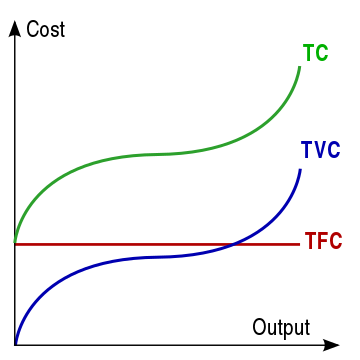
Short-run variable and fixed cost curves (SRVC and SRFC or VC and FC)

Since short-run fixed cost (FC/SRFC) does not vary with the level of output, its curve is horizontal as shown here. Short-run variable costs (VC/SRVC) increase with the level of output, since the more output is produced, the more of the variable input(s) needs to be used and paid for.

Short-run average variable cost curve (AVC or SRAVC)

Average variable cost (AVC/SRAVC) (which is a short-run concept) is the variable cost (typically labor cost) per unit of output: SRAVC = wL / Q where w is the wage rate, L is the quantity of labor used, and Q is the quantity of output produced. The SRAVC curve plots the short-run average variable cost against the level of output and is typically drawn as U-shaped. However, whilst this is convenient for economic theory, it has been argued that it bears little relationship to the real world. Some estimates show that, at least for manufacturing, the proportion of firms reporting a U-shaped cost curve is in the range of 5 to 11 percent.

Short-run average fixed cost curve (SRAFC)

Since fixed cost by definition does not vary with output, short-run average fixed cost (SRAFC) (that is, short-run fixed cost per unit of output) is lower when output is higher, giving rise to the downward-sloped curve shown.

Short-run and long-run average total cost curves (SRATC or SRAC and LRATC or LRAC)

The average total cost curve is constructed to capture the relation between cost per unit of output and the level of output, ceteris paribus. A perfectly competitive and productively efficient firm organizes its factors of production in such a way that the usage of the factors of production is as low as possible consistent with the given level of output to be produced. In the short run, when at least one factor of production is fixed, this occurs at the output level where it has enjoyed all possible average cost gains from increasing production. This is at the minimum point in the above diagram.

STC = Pk*K + PL*L

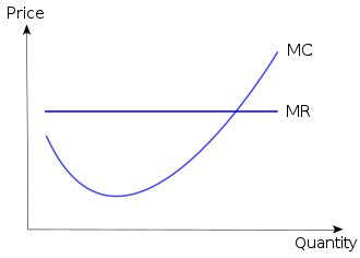
Short-run marginal cost curve (SRMC)

A short-run marginal cost (SRMC) curve graphically represents the relation between marginal (i.e., incremental) cost incurred by a firm in the short-run production of a good or service and the quantity of output produced. This curve is constructed to capture the relation between marginal cost and the level of output, holding other variables, like technology and resource prices, constant. The marginal cost curve is usually U-shaped. Marginal cost is relatively high at small quantities of output; then as production increases, marginal cost declines, reaches a minimum value, then rises. The marginal cost is shown in relation to marginal revenue (MR), the incremental amount of sales revenue that an additional unit of the product or service will bring to the firm. This shape of the marginal cost curve is directly attributable to increasing, then decreasing marginal returns (and the law of diminishing marginal returns). Marginal cost equals w/MPL. For most production processes the marginal product of labour initially rises, reaches a maximum value and then continuously falls as production increases. Thus, marginal cost initially falls, reaches a minimum value and then increases. The marginal cost curve intersects both the average variable cost curve and (short-run) average total cost curve at their minimum points. When the marginal cost curve is above an average cost curve the average curve is rising. When the marginal costs curve is below an average curve the average curve is falling. This relation holds regardless of whether the marginal curve is rising or falling.

Long-run marginal cost curve (LRMC)

The long-run marginal cost (LRMC) curve shows for each unit of output the added total cost incurred in the long run, that is, the conceptual period when all factors of production are variable. Stated otherwise, LRMC is the minimum increase in total cost associated with an increase of one unit of output when all inputs are variable.

The long-run marginal cost curve is shaped by returns to scale, a long-run concept, rather than the law of diminishing marginal returns, which is a short-run concept. The long-run marginal cost curve tends to be flatter than its short-run counterpart due to increased input flexibility. The long-run marginal cost curve intersects the long-run average cost curve at the minimum point of the latter. When long-run marginal cost is below long-run average cost, long-run average cost is falling (as additional units of output are considered).  When long-run marginal cost is above long run average cost, average cost is rising. Long-run marginal cost equals short run marginal-cost at the least-long-run-average-cost level of production. LRMC is the slope of the LR total-cost function.