Range and co-efficient of Range

The Range of a distribution gives a measure of the width (or the spread) of the data values of the corresponding random variable. For example, if there are two random variables X and Y such that X corresponds to the age of human beings and Y corresponds to the age of turtles, we know from our general knowledge that the variable corresponding to the age of turtles should be larger.

Since the average age of humans is 50-60 years, while that of turtles is about 150-200 years; the values taken by the random variable Y are indeed spread out from 0 to at least 250 and above; while those of X will have a smaller range. Thus, qualitatively you’ve already understood what the Range of a distribution means. The mathematical formula for the same is given as:

Range=L–S

where L: The largets/maximum value attained by the random variable under consideration

S: The smallest/minimum value.

Properties

• The Range of a given distribution has the same units as the data points.
• If a random variable is transformed into a new random variable by a change of scale and a shift of origin as:

Y = aX + b

where

Y: the new random variable

X: the original random variable

a,b: constants.

Then the ranges of X and Y can be related as:

R_Y = |a|R_X

Clearly, the shift in origin doesn’t affect the shape of the distribution, and therefore its spread (or the width) remains unchanged. Only the scaling factor is important.

• For a grouped class distribution, the Range is defined as the difference between the two extreme class boundaries.
• A better measure of the spread of a distribution is the Coefficient of Range, given by:

Coefficient of Range (expressed as a percentage) =L–SL+S×100

Clearly, we need to take the ratio between the Range and the total (combined) extent of the distribution. Besides, since it is a ratio, it is dimensionless, and can, therefore, one can use it to compare the spreads of two or more different distributions as well.

• The range is an absolute measure of Dispersion of a distribution while the Coefficient of Range is a relative measure of dispersion.

Due to the consideration of only the end-points of a distribution, the Range never gives us any information about the shape of the distribution curve between the extreme points. Thus, we must move on to better measures of dispersion. One such quantity is Mean Deviation which is we are going to discuss now.

The interquartile range (IQR)

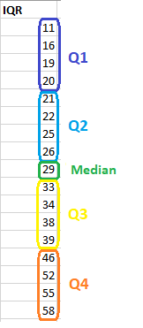
The interquartile range is the middle half of the data. To visualize it, think about the median value that splits the dataset in half. Similarly, you can divide the data into quarters. Statisticians refer to these quarters as quartiles and denote them from low to high as Q1, Q2, Q3, and Q4. The lowest quartile (Q1) contains the quarter of the dataset with the smallest values. The upper quartile (Q4) contains the quarter of the dataset with the highest values. The interquartile range is the middle half of the data that is in between the upper and lower quartiles. In other words, the interquartile range includes the 50% of data points that fall in Q2 and

The IQR is the red area in the graph below.

The interquartile range is a robust measure of variability in a similar manner that the median is a robust measure of central tendency. Neither measure is influenced dramatically by outliers because they don’t depend on every value. Additionally, the interquartile range is excellent for skewed distributions, just like the median. As you’ll learn, when you have a normal distribution, the standard deviation tells you the percentage of observations that fall specific distances from the mean. However, this doesn’t work for skewed distributions, and the IQR is a great alternative.

I’ve divided the dataset below into quartiles. The interquartile range (IQR) extends from the low end of Q2 to the upper limit of Q3. For this dataset, the range is 21 – 39.