Comparative analysis of all measures of central Tendency

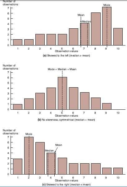
The mean, median, and mode are all useful measures of central tendency, but their value can be limited by unique characteristics of the underlying data. A comparison across alternate measures is useful for determining the extent to which a consistent pattern of central tendency emerges. If the mean, median, and mode all coincide at a single sample observation, the sample data are said to be symmetrical. If the data are perfectly symmetrical, then the distribution of data above the mean is a perfect mirror image of the data distribution below the mean. A perfectly symmetrical distribution is illustrated in Figure. Whereas a symmetrical distribution implies balance in sample dispersion, skewness implies a lack of balance. If the greater bulk of sample observations are found to the left of the sample mean, then the sample is said to be skewed downward or to the left as in Figure. If the greater bulk of sample observations are found to the right of the mean, then the sample is said to be skewed upward or to the right as in Figure). When alternate measures of central tendency converge on a single value or narrow range of values, managers can be confident that an important characteristic of a fairly homogeneous sample of observations has been discovered. When alternate measures of central tendency fail to converge on a single value or range of values, then it is likely that underlying data comprise a heterogeneous sample of observations with important subsample differences. A comparison of alternate measures of central tendency is usually an important first step to determining whether a more detailed analysis of subsample differences is necessary.

The Mean, Median, and Mode

Short Run Analysis with Law of Variable Proportion

Law of Variable Proportions occupies an important place in economic theory. This law is also known as Law of Proportionality.

Keeping other factors fixed, the law explains the production function with one factor variable. In the short run when output of a commodity is sought to be increased, the law of variable proportions comes into operation.

Therefore, when the number of one factor is increased or decreased, while other factors are constant, the proportion between the factors is altered. For instance, there are two factors of production viz., land and labour.

Land is a fixed factor whereas labour is a variable factor. Now, suppose we have a land measuring 5 hectares. We grow wheat on it with the help of variable factor i.e., labour. Accordingly, the proportion between land and labour will be 1: 5. If the number of laborers is increased to 2, the new proportion between labour and land will be 2: 5. Due to change in the proportion of factors there will also emerge a change in total output at different rates. This tendency in the theory of production called the Law of Variable Proportion.

Definitions

“As the proportion of the factor in a combination of factors is increased after a point, first the marginal and then the average product of that factor will diminish.” – Benham

“An increase in some inputs relative to other fixed inputs will in a given state of technology cause output to increase, but after a point the extra output resulting from the same additions of extra inputs will become less and less.” – Samuelson

“The law of variable proportion states that if the inputs of one resource is increased by equal increment per unit of time while the inputs of other resources are held constant, total output will increase, but beyond some point the resulting output increases will become smaller and smaller.” – Leftwitch

Assumptions

Law of variable proportions is based on following assumptions:

(i) Constant Technology

The state of technology is assumed to be given and constant. If there is an improvement in technology the production function will move upward.

(ii) Factor Proportions are Variable

The law assumes that factor proportions are variable. If factors of production are to be combined in a fixed proportion, the law has no validity.

(iii) Homogeneous Factor Units

The units of variable factor are homogeneous. Each unit is identical in quality and amount with every other unit.

(iv) Short-Run

The law operates in the short-run when it is not possible to vary all factor inputs.

Explanation of the Law

In order to understand the law of variable proportions we take the example of agriculture. Suppose land and labour are the only two factors of production.

By keeping land as a fixed factor, the production of variable factor i.e., labour can be shown with the help of the following table:

From the table 1 it is clear that there are three stages of the law of variable proportion. In the first stage average production increases as there are more and more doses of labour and capital employed with fixed factors (land). We see that total product, average product, and marginal product increases but average product and marginal product increases up to 40 units. Later on, both start decreasing because proportion of workers to land was sufficient and land is not properly used. This is the end of the first stage.

The second stage starts from where the first stage ends or where AP=MP. In this stage, average product and marginal product start falling. We should note that marginal product falls at a faster rate than the average product. Here, total product increases at a diminishing rate. It is also maximum at 70 units of labour where marginal product becomes zero while average product is never zero or negative.

The third stage begins where second stage ends. This starts from 8th unit. Here, marginal product is negative and total product falls but average product is still positive. At this stage, any additional dose leads to positive nuisance because additional dose leads to negative marginal product.

Graphic Presentation

In fig. 1, on OX axis, we have measured number of labourers while quantity of product is shown on OY axis. TP is total product curve. Up to point ‘E’, total product is increasing at increasing rate. Between points E and G it is increasing at the decreasing rate. Here marginal product has started falling. At point ‘G’ i.e., when 7 units of labourers are employed, total product is maximum while, marginal product is zero. Thereafter, it begins to diminish corresponding to negative marginal product. In the lower part of the figure MP is marginal product curve.
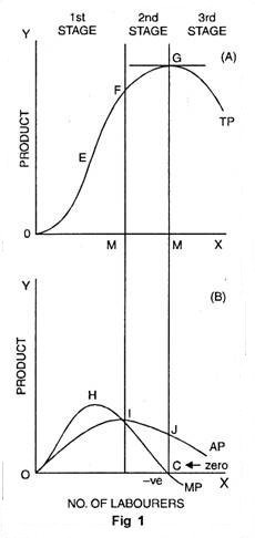
Up to point ‘H’ marginal product increases. At point ‘H’, i.e., when 3 units of labourers are employed, it is maximum. After that, marginal product begins to decrease. Before point ‘I’ marginal product becomes zero at point C and it turns negative. AP curve represents average product. Before point ‘I’, average product is less than marginal product. At point ‘I’ average product is maximum. Up to point T, average product increases but after that it starts to diminish.

Three Stages of the Law

  1. First Stage

First stage starts from point ‘O’ and ends up to point F. At point F average product is maximum and is equal to marginal product. In this stage, total product increases initially at increasing rate up to point E. between ‘E’ and ‘F’ it increases at diminishing rate. Similarly marginal product also increases initially and reaches its maximum at point ‘H’. Later on, it begins to diminish and becomes equal to average product at point T. In this stage, marginal product exceeds average product (MP > AP).

  1. Second Stage

It begins from the point F. In this stage, total product increases at diminishing rate and is at its maximum at point ‘G’ correspondingly marginal product diminishes rapidly and becomes ‘zero’ at point ‘C’. Average product is maximum at point ‘I’ and thereafter it begins to decrease. In this stage, marginal product is less than average product (MP < AP).

  1. Third Stage

This stage begins beyond point ‘G’. Here total product starts diminishing. Average product also declines. Marginal product turns negative. Law of diminishing returns firmly manifests itself. In this stage, no firm will produce anything. This happens because marginal product of the labour becomes negative. The employer will suffer losses by employing more units of labourers. However, of the three stages, a firm will like to produce up to any given point in the second stage only.

In Which Stage Rational Decision is Possible

To make the things simple, let us suppose that, a is variable factor and b is the fixed factor. And a1, a2 , a3….are units of a and b1 b2b3…… are unit of b.

Stage I is characterized by increasing AP, so that the total product must also be increasing. This means that the efficiency of the variable factor of production is increasing i.e., output per unit of a is increasing. The efficiency of b, the fixed factor, is also increasing, since the total product with b1 is increasing.

The stage II is characterized by decreasing AP and a decreasing MP, but with MP not negative. Thus, the efficiency of the variable factor is falling, while the efficiency of b, the fixed factor, is increasing, since the TP with b1 continues to increase.

Finally, stage III is characterized by falling AP and MP, and further by negative MP. Thus, the efficiency of both the fixed and variable factor is decreasing.

Rational Decision

Stage II becomes the relevant and important stage of production. Production will not take place in either of the other two stages. It means production will not take place in stage III and stage I. Thus, a rational producer will operate in stage II.

Suppose b were a free resource; i.e., it commanded no price. An entrepreneur would want to achieve the greatest efficiency possible from the factor for which he is paying, i.e., from factor a. Thus, he would want to produce where AP is maximum or at the boundary between stage I and II.

If on the other hand, a were the free resource, then he would want to employ b to its most efficient point; this is the boundary between stage II and III.

Obviously, if both resources commanded a price, he would produce somewhere in stage II. At what place in this stage production takes place would depend upon the relative prices of a and b.

Condition or Causes of Applicability

There are many causes which are responsible for the application of the law of variable proportions.

They are as follows:

  1. Under Utilization of Fixed Factor

In initial stage of production, fixed factors of production like land or machine, is under-utilized. More units of variable factor, like labour, are needed for its proper utilization. As a result of employment of additional units of variable factors there is proper utilization of fixed factor. In short, increasing returns to a factor begins to manifest itself in the first stage.

  1. Fixed Factors of Production

The foremost cause of the operation of this law is that some of the factors of production are fixed during the short period. When the fixed factor is used with variable factor, then its ratio compared to variable factor falls. Production is the result of the co-operation of all factors. When an additional unit of a variable factor has to produce with the help of relatively fixed factor, then the marginal return of variable factor begins to decline.

  1. Optimum Production

After making the optimum use of a fixed factor, then the marginal return of such variable factor begins to diminish. The simple reason is that after the optimum use, the ratio of fixed and variable factors become defective. Let us suppose a machine is a fixed factor of production. It is put to optimum use when 4 labourers are employed on it. If 5 labourers are put on it, then total production increases very little and the marginal product diminishes.

  1. Imperfect Substitutes

Mrs. Joan Robinson has put the argument that imperfect substitution of factors is mainly responsible for the operation of the law of diminishing returns. One factor cannot be used in place of the other factor. After optimum use of fixed factors, variable factors are increased and the amount of fixed factor could be increased by its substitutes.

Such a substitution would increase the production in the same proportion as earlier. But in real practice factors are imperfect substitutes. However, after the optimum use of a fixed factor, it cannot be substituted by another factor.

Applicability of the Law of Variable Proportions:

The law of variable proportions is universal as it applies to all fields of production. This law applies to any field of production where some factors are fixed and others are variable. That is why it is called the law of universal application.

The main cause of application of this law is the fixity of any one factor. Land, mines, fisheries, and house building etc. are not the only examples of fixed factors. Machines, raw materials may also become fixed in the short period. Therefore, this law holds good in all activities of production etc. agriculture, mining, manufacturing industries.

  1. Application to Agriculture

With a view of raising agricultural production, labour and capital can be increased to any extent but not the land, being fixed factor. Thus when more and more units of variable factors like labour and capital are applied to a fixed factor then their marginal product starts to diminish and this law becomes operative.

  1. Application to Industries

In order to increase production of manufactured goods, factors of production has to be increased. It can be increased as desired for a long period, being variable factors. Thus, law of increasing returns operates in industries for a long period. But, this situation arises when additional units of labour, capital and enterprise are of inferior quality or are available at higher cost.

As a result, after a point, marginal product increases less proportionately than increase in the units of labour and capital. In this way, the law is equally valid in industries.

Postponement of the Law

The postponement of the law of variable proportions is possible under following conditions:

(i) Improvement in Technique of Production

The operation of the law can be postponed in case variable factors techniques of production are improved.

(ii) Perfect Substitute

The law of variable proportion can also be postponed in case factors of production are made perfect substitutes i.e., when one factor can be substituted for the other.

Short Run Production Function with Two Variable Inputs

For the analysis of production function with two variable factors we make use of the concept called isoquants or iso-product curves which are similar to indifference curves of the theory of demand. Therefore, before we explain the production function with two variable factors and returns to scale, we shall explain the concept of isoquants (that is, equal product curves) and their properties.

Isoquants

Isoquants, which are also called equal product curves, are similar to the indifference curves of the theory of consumer’s behaviour. An isoquant represents all those factor combinations which are capable of producing the same level of output.

The isoquants are thus contour lines which trace the loci of equal outputs. Since an isoquant represents those combinations of inputs which will be ca­pable of producing an equal quantity of output, the producer would be indifferent between them. Therefore, isoquants are also often called equal product curves production-indifference curves.

Table 1. Factor Combinations to Produce a Given or Level of Output:

The concept of isoquant can be easily understood from Table 1. It is presumed that two factors labour and capital are being employed to produce a product. Each of the factor combinations A. B, C, D and E produces the same level of output, say 100 units. To start with, factor combination A consisting of 1 unit of labour and 12 units of capital produces the given 100 units of output.

Similarly, combination B consisting of 2 units of labour and 8 units of capital, combination C con­sisting of 3 units of labour and 5 units of capital, combination D consisting of 4 units of labour and 3 units of capital, combination E consisting of 5 units of labour and 2 units of capital are capable of producing the same amount of output, i.e., 100 units. In Fig. 1 we have plotted all these combinations and by joining them we obtain an isoquant showing that every combination repre­sented on it can produce 100 units of output.

Isoquants Though isoquants are similar to be indifference curves of the theory of consumer’s behaviour, there is one important difference between the two. An indifference curve represents all those combi­nations of two goods which provide the same satisfaction or utility to a consumer but no attempt is made to specify the level of utility in exact quantitative terms it stands for.

This is so because the cardinal measurement of satisfaction or utility in unambiguous thermos is not possible. That is why we usually label indifference curves by ordinal numbers as I, II, III etc. indicating that a higher indiffer­ence curve represents a higher level of satisfaction than a lower one, but the information as to how much one level of satisfaction is greater than another is not provided.

On the other hand, we can label isoquants in the physical units of output without any difficulty. Production of a good being a physical phenomenon lends itself easily to absolute measurement in physical units. Since each isoquant represents a specified level of production, it is possible to say by how much one isoquant indicates greater or less production than another.

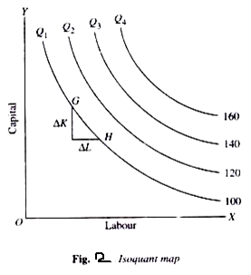
In Fig. 2 we have drawn an isoquant-map or equal- product map with a set of four isoquants which represent 100 units, 120 units, 140 units and 160 units of output respectively. Then, from this set of isoquants it is very easy to judge by how much production level on one isoquant curve is greater or less than on another.

Ridge Lines

The marginal product of a particular factor may be negative if the quantity used is too large. For example, if too much labour is used there may be congestion and the efficiency of all the labourers may be affected. An isoquant will include points denoting such factor quantities, because it includes all factor combinations producing the same output.

But, a rational producer will not operate on this part of the isoquant. The area of rational operation may be shown by drawing two lines from the ori­gin enclosing only those parts of the isoquants where each factor has a positive marginal product. Such lines are called ridge lines. Negative marginal products appear in that part of the isoquant which has a posi­tive slope.

Ridge lines exclude these parts. This can be seen in Fig. 3. Let us focus our atten­tion on isoquant Q1 over the interval from point A to point E. We now know that as we substitute labour for capital and move from A toward E, the marginal productivity of labour diminishes.

But, look what happens if we move beyond E, continuing to use more labour. The isoquant Q1 turns upward, indicating that if we use more labour and still want to produce Q1 units, we must now also use more capital. Why? Because beyond E, the marginal product of labour has become negative, and so to compensate for using more labour, we must add to the amount of capital used as well.

If we follow Q2, Q3 or Q4 from left to right, we see that a similar result occurs. Beyond points F, G and H turn up. That is, the slopes of the isoquants become positive due to the negative marginal productivity of labour.

The line (R’) connecting all points, such as £, F, G and H, is called a ridge line; it marks off the boundary between stage II and stage III of production. No one would want to produce in stage III, since the same level of production could be obtained with fewer of both inputs by moving to the left along the appropriate isoquant until stage II was reached.

We can now apply this same line of reasoning to rule out stage I. Again let us concentrate attention on isoquant Q1. This time, suppose we move up and to the left toward point A. As we do so, substituting capital for labour, the marginal productivity of capital diminishes and becomes negative if we go beyond A. Thus, if we add more capital above A while maintaining output at the Q1 level, we must use more labour.

This does not make much sense from a managerial perspective. Points B, C and D are analogous to point A for their respective isoquants. Beyond these points, the marginal productivity of capital is negative and so we would not wish to operate in that region, which we refer to as stage I.

The ridge line R marks the boundary between stage I and stage II just as R’ marks the boundary between stages II and III. We see that neither stage I nor stage III is desirable for production, since the marginal productivity of at least one input is negative in those stages. We can then conclude that the only relevant region for production is stage II, which is bounded by the two ridge lines, R1 and R2. This region is called the economic region of produc­tion.

Least Cost Combination of Inputs

The firm may produce a particular quantity of its product at each of the alternative input combinations that lies on the IQ for that quantity. Since the firm’s goal is to maximize profit, the optimum input combination for producing a particular quantity of its product would be one that would produce the output at the minimum possible cost.

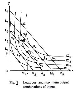
The optimum input combination in this case is known as the least cost combination of inputs. In order to explain the firm’s selection of the least cost combination of inputs, let us suppose that some of the firm’s isoquants (IQs) and iso-cost lines (ICLs) are given in Fig. 1.

Let us now suppose that the firm intends to produce a particular quantity q = q3 of its product, and the isoquant for this particular quantity is IQ3. In other words, if the firm uses any of the input combinations lying on IQ3, it would be able to produce the output quantity q = q3.

But, since the different points on IQ3, viz., S1, S2, S3, S4, S5, etc. lie on different ICLs, they produce the same output, viz., q = but at different levels of cost, For we know that a higher (or a lower) ICL represents a higher (or a lower) level of cost.

Therefore, in order to produce the output of q3 at the least possible cost, the firm would have to select that point on IQ3 that would lie on the lowest possible ICL. In Fig. 8.12, we see that the point S3 on IQlies on the lowest possible ICL, viz., L3M3. Any other point on IQ3 lies on a higher ICL or a higher level of cost than L3M3.

Therefore, at an output of q3, the least cost combination of inputs is S3(x̅, y̅). In other words, if the firm is to produce an output of q3, it would buy and use the quantity x of input X and the quantity y of input Y. Here it is very important for us to observe that the least cost combination of inputs is the point of tangency (here S3) between the particular isoquant (here IQ3) and an iso-cost line (here L3M3).

Similarly, for producing a particular quantity of output, if the firm is to remain on IQ2, then the least cost combination of inputs would be given by the point T2, because this point is the point of tangency between IQ2 and an ICL (i.e., L2M2).

Maximum Output Combination of Inputs

In iso-cost lines (ICLs), we have seen that if the prices (rX and rY) of the inputs (X and Y) are given and constant, then by spending a particular amount of money the firm can buy any one of a large number of input combinations that lie on the corresponding ICL.

Since the firm’s goal is to maximize the level of profit, the optimum input combination in this case would be one that would produce the maximum possible output. Therefore, this input combination is called the maximum- output combination of inputs.

We shall now see with the help of Fig. 8.12, how the maximum output-input combination can be obtained by the firm. Let us suppose that the firm has decided to spend a particular amount of money, TVC3, (TVC stands for total variable cost) for the two variable inputs (X and Y), and the ICL for this expenditure is L3M3.

That is, if the firm is to spend the amount of money TVC3, then it would have to buy some combination that lie on the iso-cost line, L3M3.

Now the points like V1, V2 S3, V4, V5 lying on L3M3 are situated on different isoquants. That is, at different points on the line L3M3, the cost of the firm is the same (= TVC3), but the quantities produced are different.

Since a higher IQ represents a higher level of output, of all the points on L3M3, the profit-maximizing firm would select that one as optimum which lies on the highest possible IQ, i.e., which produces the highest possible level of output. This point is S(x̅, y̅) on, IQ3—this point is the maximum-output Combination of inputs subject to the cost constraint of TVC = TVC3.

We have to note here that the maximum-output combination of inputs subject to the cost constraint (here S3) is the point of tangency between the ICL corresponding to the given cost level (here TVC3) and an IQ (here IQ3).

Similarly, if the given ICL of the firm is L4M4, then the maximum-output combination of inputs would be the point R4, because this point is the point of tangency between the line L4M4 and an IQ which is here IQ4.

Long Run Production Function

Production in the short run in which the functional relationship between input and output is explained assuming labor to be the only variable input, keeping capital constant.

In the long run production function, the relationship between input and output is explained under the condition when both, labor and capital, are variable inputs.

In the long run, the supply of both the inputs, labor and capital, is assumed to be elastic (changes frequently). Therefore, organizations can hire larger quantities of both the inputs. If larger quantities of both the inputs are employed, the level of production increases. In the long run, the functional relationship between changing scale of inputs and output is explained under laws of returns to scale. The laws of returns to scale can be explained with the help of isoquant technique.

Isoquant Curve

The relationships between changing input and output is studied in the laws of returns to scale, which is based on production function and isoquant curve. The term isoquant has been derived from a Greek work iso, which means equal. Isoquant curve is the locus of points showing different combinations of capital and labor, which can be employed to produce same output.

It is also known as equal product curve or production indifference curve. Isoquant curve is almost similar to indifference curve. However, there are two dissimilarities between isoquant curve and indifference curve. Firstly, in the graphical representation, indifference curve takes into account two consumer goods, while isoquant curve uses two producer goods. Secondly, indifference curve measures the level of satisfaction, while isoquant curve measures output.

Some of the popular definitions of isoquant curve are as follows:

According to Ferguson, “An isoquant is a curve showing all possible combinations of inputs physically capable of producing a given level of output.”

According to Peterson, “An isoquant curve may be defined as a curve showing the possible combinations of two variable factors that can be used to produce the same total product”

From the aforementioned definitions, it can be concluded that the isoquant curve is generated by plotting different combinations of inputs on a graph. An isoquant curve provides the best combination of inputs at which the output is maximum.

Following are the assumptions of isoquant curve:

  • Assumes that there are only two inputs, labor and capital, to produce a product
  • Assumes that capital, labor, and good are divisible in nature
  • Assumes that capital and labor are able to substitute each other at diminishing rates because they are not perfect substitutes
  • Assumes that technology of production is known

On the basis of these assumptions, isoquant curve can be drawn with the help of different combinations of capital and labor. The combinations are made such that it does not affect the output.

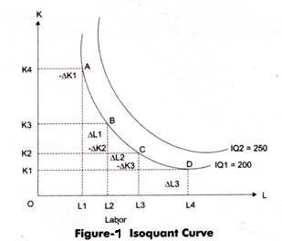
Figure-1 represents an isoquant curve for four combinations of capital and labor:

In Figure-1, IQ1 is the output for four combinations of capital and labor. Figure 1 shows that all along the curve for IQ1 the quantity of output is same that is 200 with the changing combinations of capital and labor. The four combinations on the IQ1 curve are represented by points A, B, C, and D.

Some of the properties of the isoquant curve are as follows:

  1. Negative Slope

Implies that the slope of isoquant curve is negative. This is because when capital (K) is increased, the quantity of labor (L) is reduced or vice versa, to keep the same level of output.

  1. Convex to Origin

Shows the substitution of inputs and diminishing marginal rate of technical substitution (which is discussed later) in economic region. This implies that marginal significance of one input (capital) in terms of another input (labor) diminishes along with the isoquant curve.

  1. Non-intersecting and Non-tangential

Implies that two isoquant curves (as shown in Figure-1) cannot cut each other.

  1. Upper isoquant have high output

Implies that upper curve of the isoquant curve produces more output than the curve beneath. This is because of the larger combination of input result in a larger output as compared to the curve that s beneath it. For example, in Figure-5 the value of capital at point B is greater than the capital at point C. Therefore, the output of curve Q2 is greater than the output of Q1.

Forms of Isoquants

The shape of an isoquant depends on the degree to which one input can be substituted by the other. Convex isoquant represents that there is a continuous substitution of one input variable by the other input variable at a diminishing rate.

However, in economics, there are other forms of isoquants, which are as follows:

  1. Linear Isoquant

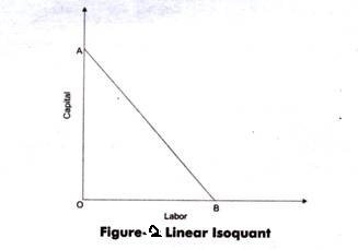
Refers to a straight line isoquant. Linear isoquant represents a perfect substitutability between the inputs, capital and labor, of the production function. It implies that a product can be produced by using either capital or labor or using both, if capital and labor are perfect substitutes of each other. Therefore, in a linear isoquant, MRTS between inputs remains constant.

The algebraic form of production function in case of linear isoquant is as follows:

Q = aK + BL

Here, Q is the weighted sum of K and L.

Slope of curve can be calculated with the help of following formula:

MPK = ∆Q/∆K = a

MPL = ∆Q/∆L = b

MRTS = MPL/MPK

MRTS = -b/a

However, linear isoquant does not have existence in the real world.

Figure-2 shows a linear isoquant

  1. L-shaped Isoquant

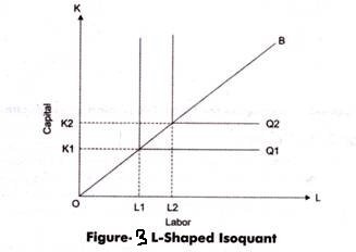
Refers to an isoquant in which the combination between capital and labor are in a fixed proportion. The graphical representation of fixed factor proportion isoquant is L in shape. The L-shaped isoquant represents that there is no substitution between labor and capital and they are assumed to be complementary goods.

It represents that only one combination of labor and capital is possible to produce a product with affixed proportion of inputs. For increasing the production, an organization needs to increase both inputs proportionately.

Figure-3 shows an L-shaped isoquant

In Figure-3, it can be seen OK1 units of capital and OL1 units of labor are required for the production of Q1. On the other hand, to increase the production from Q1 to Q2, an organization needs to increase inputs from K1 to K2 and L1 to L2 both.

This relationship between capital and labor can be expressed as follows:

Q = f (K, L) = min (aK, bL)

Where, min = Q equals to lower of the two terms, aK and bL

For example, in case aK > bL, then Q = bL and in case aK < bL then, Q = aK.

L-shaped isoquant is applied in many production activities and techniques where labor and capital is in fixed proportion. For example, in the process of driving a car, only one machine and one labor is required, which is a fixed combination.

  1. Kinked Isoquant

Refers to an isoquant that represents different combinations of labor and capital. These combinations can be used in different processes of production, but in fixed proportion. According to L-shaped isoquant, there would be only one combination between capital and labor in a fixed proportion. However, in real life, there can be several ways to perform production with different combinations of capital and labor.

For example, there are two machines in which one is large in size and can perform all the processes involved in production, while the other machine is small in size and can perform only one function of production process. In both the machines, combination of capital employed and labor used is different.

Let us understand kinked isoquant with the help of another example. For example, to produce 100 units of product X, an organization has used four different techniques of production with fixed-factor proportion.

Laws of Returns to Scale

Law of Returns to Scale explains the relationship between the proportional increase in all inputs and the resulting change in output in the long run, when all factors of production are variable.

On the basis of these possibilities, law of returns can be classified into three categories:

  • Increasing returns to scale
  • Constant returns to scale
  • Diminishing returns to scale
  1. Increasing Returns to Scale

If the proportional change in the output of an organization is greater than the proportional change in inputs, the production is said to reflect increasing returns to scale. For example, to produce a particular product, if the quantity of inputs is doubled and the increase in output is more than double, it is said to be an increasing returns to scale. When there is an increase in the scale of production, the average cost per unit produced is lower. This is because at this stage an organization enjoys high economies of scale.

Figure-1 shows the increasing returns to scale:

In Figure-1, a movement from a to b indicates that the amount of input is doubled. Now, the combination of inputs has reached to 2K+2L from 1K+1L. However, the output has Increased from 10 to 25 (150% increase), which is more than double. Similarly, when input changes from 2K-H2L to 3K + 3L, then output changes from 25 to 50(100% increase), which is greater than change in input. This shows increasing returns to scale.

There a number of factors responsible for increasing returns to scale.

Some of the factors are as follows:

(i) Technical and managerial indivisibility:

Implies that there are certain inputs, such as machines and human resource, used for the production process are available in a fixed amount. These inputs cannot be divided to suit different level of production. For example, an organization cannot use the half of the turbine for small scale of production.

Similarly, the organization cannot use half of a manager to achieve small scale of production. Due to this technical and managerial indivisibility, an organization needs to employ the minimum quantity of machines and managers even in case the level of production is much less than their capacity of producing output. Therefore, when there is increase in inputs, there is exponential increase in the level of output.

(ii) Specialization:

Implies that high degree of specialization of man and machinery helps in increasing the scale of production. The use of specialized labor and machinery helps in increasing the productivity of labor and capital per unit. This results in increasing returns to scale.

(iii) Concept of Dimensions:

Refers to the relation of increasing returns to scale to the concept of dimensions. According to the concept of dimensions, if the length and breadth of a room increases, then its area gets more than doubled.

For example, length of a room increases from 15 to 30 and breadth increases from 10 to 20. This implies that length and breadth of room get doubled. In such a case, the area of room increases from 150 (15*10) to 600 (30*20), which is more than doubled.

  1. Constant Returns to Scale

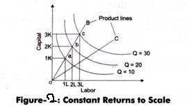
The production is said to generate constant returns to scale when the proportionate change in input is equal to the proportionate change in output. For example, when inputs are doubled, so output should also be doubled, then it is a case of constant returns to scale.

Figure-2 shows the constant returns to scale:

In Figure-2, when there is a movement from a to b, it indicates that input is doubled. Now, when the combination of inputs has reached to 2K+2L from IK+IL, then the output has increased from 10 to 20.

Similarly, when input changes from 2Kt2L to 3K + 3L, then output changes from 20 to 30, which is equal to the change in input. This shows constant returns to scale. In constant returns to scale, inputs are divisible and production function is homogeneous.

  1. Diminishing Returns to Scale

Diminishing returns to scale refers to a situation when the proportionate change in output is less than the proportionate change in input. For example, when capital and labor is doubled but the output generated is less than doubled, the returns to scale would be termed as diminishing returns to scale.

Figure 3 shows the diminishing returns to scale:

In Figure-3, when the combination of labor and capital moves from point a to point b, it indicates that input is doubled. At point a, the combination of input is 1k+1L and at point b, the combination becomes 2K+2L.

However, the output has increased from 10 to 18, which is less than change in the amount of input. Similarly, when input changes from 2K+2L to 3K + 3L, then output changes from 18 to 24, which is less than change in input. This shows the diminishing returns to scale.

Diminishing returns to scale is due to diseconomies of scale, which arises because of the managerial inefficiency. Generally, managerial inefficiency takes place in large-scale organizations. Another cause of diminishing returns to scale is limited natural resources. For example, a coal mining organization can increase the number of mining plants, but cannot increase output due to limited coal reserves.

Expansion Path

In economics, an expansion path (also called a scale line) is a curve in a graph with quantities of two inputs, typically physical capital and labor, plotted on the axes. The path connects optimal input combinations as the scale of production expands. A producer seeking to produce a given number of units of a product in the cheapest possible way chooses the point on the expansion path that is also on the isoquant associated with that output level.

Economists Alfred Stonier and Douglas Hague defined “expansion path” as “that line which reflects the least–cost method of producing different levels of output, when factor prices remain constant.” The points on an expansion path occur where the firm’s isocost curves, each showing fixed total input cost, and its isoquants, each showing a particular level of output, are tangent; each tangency point determines the firm’s conditional factor demands. As a producer’s level of output increases, the firm moves from one of these tangency points to the next; the curve joining the tangency points is called the expansion path.

If an expansion path forms a straight line from the origin, the production technology is considered homothetic (or homoethetic). In this case, the ratio of input usages is always the same regardless of the level of output, and the inputs can be expanded proportionately so as to maintain this optimal ratio as the level of output expands. A Cobb–Douglas production function is an example of a production function that has an expansion path which is a straight line through the origin.

Meaning of Expansion Path:

We know that the production function of the firm

q = f(x,y)

Gives us the isoquant map of the firm, one isoquant (IQ) for each particular level of output, and the cost equation of the firm

C = rXx + rYy           

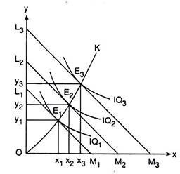
gives us the family of parallel iso-cost lines (ICLs), given the prices of the inputs rX and rY, one ICL for one particular level of cost. The IQ-map and the family of ICLs have been given in Fig. If we now join the point of origin 0 and the points of tangency, E1, E2, E3, etc., between the IQs and the ICLs by a curve, then this curve would give us what is known as the expansion path of the firm.

The expansion path is so called because if the firm decides to expand its operations, it would have to move along this path. Let us note that the firm may expand in two ways.

First, it may want to expand by successively increasing its level of cost or its expenditure on the inputs X and Y, i.e., by using more and more of inputs, and, consequently, by producing more of its output.

Second, the firm may decide to expand by increasing its level of output per period. This the firm may do by increasing the expenditure on the inputs, i.e., by using more and more of them.

The two approaches to expansion apparently appear to be the same, for both involve an increase in expenditure. However, there is a fundamental difference. In the first case, decision is taken initially at the point of cost. Cost levels are made higher and higher and then efforts are made to maximize the level of output subject to the cost constraint.

On the other hand, in the second case, decision-making occurs initially and directly at the point of output. Here the firm first decides to produce more of output and then efforts are made to produce the output at the minimum possible cost.

Types of Expansion Path

  1. Expansion by Means of Increasing the Level of Expenditure on the Inputs

In Fig. let us suppose that, initially, the firm’s level of cost is such that its ICL is L1M1 and output-maximization subject to cost constraint occurs at the point of tangency, E1, between the ICL, L1M1, and an IQ which is IQ1. At E1 the firm uses X1 of the first input and y1 of the second input to produce the maximum possible output, say, q1, which is represented by IQ1.

Now, if the firm decides to expand by increasing the cost level from the level of L1M1 to that of L2M2, then the firm would be in output-maximising equilibrium at the point of tangency E2 (x2, y2), on IQ2, using more of the inputs, x2 > x1 and y2 > y1, and producing an output level, say, q2, q2 > q1, since IQ2 is a higher isoquant than IQ1.

In the same way, if the firm decides to expand further, it would increase its cost level from that of L2M2 to that of L3Mand it would produce the maximum output subject to the cost constraint at the point of tangency E3 (x3, y3) on IQ3 using more of the inputs, x3 > x2 and y3 > y2, and producing a higher level of output, say, q3, q3 > q2, since IQ3 is a higher IQ than IQ2.

The process of expansion of firm’s operations through increases in the level of cost may go on in this say so long as the firm decides in its favour. If we now join the point of origin O and the points E1, E2, E3, etc. by a path, then we would obtain the firm’s expansion path.

That is, if the firm expands by increasing its level of cost, it would have to move successively from one equilibrium point to another along this expansion path.

We have joined the path through the equilibrium points E1, E2, etc. with the point of origin O, because if the firm moves backward along the expansion path by decreasing the cost level then it would be moving from the initial equilibrium point, say, E3 to E2, then from E2 to E) and would approach the point O which would be the limiting point in this process.

As the firm’s cost level decreases and tends to zero, the input quantities and the output quantity would all decrease and tend to zero, and thus the point of origin O would be the limiting point.

  1. Expansion by Means of Increasing the Level of Output

In Fig. let us suppose that initially the firm decides to produce q1 of output which can be produced at any point on the isoquant, IQ1. The firm would be in cost-minimizing equilibrium at the point E1 which is the point of tangency between IQ1 and an iso-cost line say, ICL1. At the point E1, the firm would use Xi and y] quantities of the two inputs and its cost amounts to, say, C1, which is the minimum possible.

The firm may now decide to expand by increasing its level of output from q1 to q2 on IQ2. If the firm makes this decision, its cost-minimizing equilibrium will be obtained at the point of tangency E2 (x2, y2) on L2M2 using more of the inputs, x2 > x1 and y2 > y1 and incurring a cost level C2 on L2M2, which is the minimum possible required to produce the output of q2. However, C2 > C1 since L2M2 is a higher ICL than L2M2.

In the same way, the firm may decide to increase again its level of output from q2 to q3 on IQ3. In this case, the firm’s equilibrium point would be the point of tangency E3 (x3, y3) on the ICL, L3M3. At E3, the firm would use still more of the inputs, x3 > x2 and y3 > y2, incurring a cost level C3 on L3M3, which is the minimum required for producing q3 of output. However, C3 > C2 since L3M3 is a higher ICL than L2M2.

The firm’s process of expansion may go on like this as long as it decides to expand. The expansion path again would be OK that would start from the point of origin O and pass through the points E1, E2, E3, etc.

If the firm decides to contract and produce less of output, then the limiting point of the process of contraction would be the point of origin O, where the firm’s use of the inputs, its cost level and output would all tend to zero.

The Equation of the Expansion Path

Each point on the expansion path, is a point of tangency between an isoquant and an iso-cost line. Therefore, at each point on the expansion path, we have numerical slope of the IQ = numerical slope of the ICL

 MRTSX,Y = rX/rY

 fX/fY= rX/rY = constant [... rX and rY are given and constant]

Therefore, gives us the equation of the expansion path.

Economies and Diseconomies of Scale

Economies and diseconomies of scale are concepts that describe the relationship between a firm’s output and the cost of production. These phenomena help businesses understand how increasing or decreasing the scale of production affects efficiency, cost, and overall profitability. They are central to business decision-making, influencing production strategies, pricing, and competitive advantage.

Economies of Scale

Economies of scale refer to the cost advantages that a firm experiences as it increases its scale of production. As the scale of production grows, the average cost per unit of output generally decreases. This reduction in cost arises from various factors that enable businesses to spread fixed costs over a larger number of units and improve efficiency.

Types of Economies of Scale

  • Technical Economies: These arise from the use of specialized machinery, technologies, and advanced techniques in production. As firms expand, they can afford to invest in more efficient, high-capacity equipment, reducing the cost of production per unit.
    • Example: A car manufacturer investing in automated production lines that can produce cars more efficiently than manual labor.
  • Purchasing Economies: As firms increase their scale, they can negotiate better deals with suppliers for bulk purchases of raw materials and components. This allows them to reduce the per-unit cost of inputs.
    • Example: A large retailer buying products in bulk, securing discounts from suppliers.
  • Managerial Economies: Larger firms can afford to hire specialists and managers for specific tasks, which improves productivity and reduces the costs associated with less skilled or generalist workers. This leads to more effective decision-making and management.
    • Example: A multinational company employing a team of experts in areas like marketing, logistics, and finance, improving overall efficiency.
  • Financial Economies: Bigger firms often have better access to credit and can secure financing at lower interest rates. Financial institutions are more willing to lend to large, established companies, reducing their borrowing costs.
    • Example: A large corporation securing loans at a lower interest rate than a small startup.
  • Marketing Economies: Larger firms benefit from spreading their advertising and marketing costs over a larger volume of output. With a bigger customer base, the cost of reaching each individual consumer is reduced.
    • Example: A large multinational corporation advertising globally, with the cost of marketing distributed across various markets.

Benefits of Economies of Scale

  • Lower per-unit cost:

The most significant benefit of economies of scale is the reduction in average cost per unit as production increases.

  • Competitive Advantage:

Firms with lower production costs can offer products at more competitive prices, increasing market share and profitability.

  • Increased Profitability:

Reduced costs lead to improved profit margins, even if product prices remain constant.

Diseconomies of Scale

Diseconomies of scale refer to the rise in per-unit costs as a firm becomes too large. After a certain point, increasing the scale of production can lead to inefficiencies, reducing the benefits gained from economies of scale. Diseconomies of scale usually occur when a firm becomes too complex or difficult to manage, causing a decrease in efficiency.

Causes of Diseconomies of Scale

  • Management Inefficiencies: As firms grow, the complexity of managing operations increases. Communication problems, decision-making delays, and lack of coordination can emerge. Larger firms may struggle to maintain effective management structures.
    • Example: A company with many layers of management, leading to slow decision-making and poor communication.
  • Employee Alienation: In large organizations, workers may feel less motivated and alienated due to the scale of operations. This can lead to lower productivity and higher absenteeism.
    • Example: Employees in large factories might feel less connected to the company’s goals and mission, resulting in lower morale and engagement.
  • Overextension of Resources: As firms grow, they may overuse their resources, including human capital, machinery, and raw materials, leading to inefficiencies and increased costs.
    • Example: A company expanding its production line too quickly without the necessary infrastructure, leading to bottlenecks in the production process.
  • Increased Bureaucracy: As organizations become larger, they often become more bureaucratic. Increased rules, regulations, and procedures can slow down operations, making it harder to respond to market changes or innovate.
    • Example: A large corporation with numerous departments and rules, resulting in slower decision-making processes.

Consequences of Diseconomies of Scale

  • Higher per-unit cost: As firms experience diseconomies of scale, their cost per unit of output begins to rise rather than fall.
  • Reduced Profit Margins: Higher costs can squeeze profit margins, making it difficult for firms to remain competitive, especially in price-sensitive markets.
  • Operational Inefficiency: Over time, diseconomies of scale can cause operational disruptions, which affect product quality and customer satisfaction.

Balance Between Economies and Diseconomies of Scale

The key to successful growth for businesses lies in finding the right balance between economies and diseconomies of scale. Initially, as firms grow, they experience economies of scale, leading to cost reductions and efficiency. However, after reaching a certain level, additional growth may lead to diseconomies of scale, reducing the benefits gained from expansion.

Firms must continuously monitor their production processes, management structures, and organizational practices to avoid reaching the point of diseconomies of scale. By optimizing operations, investing in new technologies, and maintaining efficient management, firms can grow while minimizing the risks associated with diseconomies.

Cost Concept: Accounting and Economic Costs, Implicit and Explicit cost, Fixed and Variable Costs, Total Cost, Marginal Cost and Average Cost

Cost analysis is all about the study of the behavior of cost with respect to various production criteria like the scale of operations, prices of the factors of production, size of output, etc. It is all about the financial aspects of production.

Accounting and Economic Costs

When a firm starts producing goods, it has to pay the price for the factors employed for the production. These factors include wages to workers employed, prices for the raw materials, fuel and power used, rent for the building he hires, and interest on the money borrowed for doing business, etc.

Accounting Costs are these costs which are included in the cost of production. Hence, accounting costs take care of all payments and charges that the firm makes to suppliers of different productive factors.

Usually, a businessman invests some capital in his firm. If he would have invested the amount in some other firm, then he could have earned a certain interest/dividend. Further, he invests time for his business and also contributes his entrepreneurial and managerial ability to the business.

If not involved in the business, he could have offered his services to other firms for an amount of money. Accounting costs do not involve these costs. They form a part of the Economic Costs. Hence, Economic costs include:

  • The normal return on the money that the businessman invests in his own business
  • The salary not paid to the entrepreneur but could have been earned if the services would have been sold elsewhere.
  • A reward for all factors owned by the businessman and used in his own business.

Therefore, the accounting costs involve cash payments that the firm makes. Economic costs, on the other hand, include the accounting costs and also take into account the amount of money the businessman could have earned with his resources if he would not have started the business.

Another name for accounting costs is Explicit Costs. Whereas, the alternate name for the costs of factors that the businessman owns is Implicit Costs. A businessman earns profits when his revenues exceed both explicit and implicit costs.

Implicit and explicit cost

Implicit cost

An implicit cost is any cost that has already occurred but not necessarily shown or reported as a separate expense. It represents an opportunity cost that arises when a company uses internal resources toward a project without any explicit compensation for the utilization of resources. This means when a company allocates its resources, it always forgoes the ability to earn money off the use of the resources elsewhere, so there’s no exchange of cash. Put simply, an implicit cost comes from the use of an asset, rather than renting or buying it.

Implicit costs are also referred to as imputed, implied, or notional costs. These costs aren’t easy to quantify. That’s because businesses don’t necessarily record implicit costs for accounting purposes as money does not change hands.

These costs represent a loss of potential income, but not of profits. A company may choose to include these costs as the cost of doing business since they represent possible sources of income.

Explicit Cost

Explicit costs are normal business costs that appear in the general ledger and directly affect a company’s profitability. Explicit costs have clearly defined dollar amounts, which flow through to the income statement. Examples of explicit costs include wages, lease payments, utilities, raw materials, and other direct costs.

Explicit costs—also known as accounting costs—are easy to identify and link to a company’s business activities to which the expenses are attributed. They are recorded in a company’s general ledger and flow through to the expenses listed on the income statement. The net income (NI) of a business reflects the residual income that remains after all explicit costs have been paid. Explicit costs are the only accounting costs that are necessary to calculate a profit, as they have a clear impact on a company’s bottom line. The explicit-cost metric is especially helpful for companies’ long-term strategic planning.

Fixed and Variable Costs

Fixed costs or Constant costs are not a function of the output. That is, they do not vary with the output up to a certain extent. They require a fixed expenditure of funds regardless of the output.

For example, rent, property taxes, interest on loans, etc. However, note that fixed costs can vary with the size of the plant and are usually a function of capacity. Therefore, we can conclude that fixed costs do not vary with the output volume within a capacity level.

Businesses cannot avoid fixed costs and are applicable as long as the business is operating. Alternate names for fixed costs are inescapable or uncontrollable costs.

It is important to note here, that some fixed costs continue even after the suspension of business. For example, costs associated with storing of machines that the business cannot sell in the market, etc.

Variable costs are cost concepts which are a function of the output in the production period. Variable costs vary directly with the output. Some examples of variable costs are the cost of raw materials, wages, etc. Sometimes, they vary proportionally with the output too. However, these variations depend on the utilization of fixed facilities and resources during the production process.

Total Cost

In economics, the total cost (TC) is the total economic cost of production. It consists of variable costs and fixed costs. Total cost is the total opportunity cost of each factor of production as part of its fixed or variable costs.

Marginal Cost

In economics, marginal cost is the change in the total cost when the quantity produced changes by one unit. It is the cost of producing one more unit of a good. Marginal cost includes all of the costs that vary with the level of production. For example, if a company needs to build a new factory in order to produce more goods, the cost of building the factory is a marginal cost. The amount of marginal cost varies according to the volume of the good being produced. Economic factors that impact the marginal cost include information asymmetries, positive and negative externalities, transaction costs, and price discrimination. Marginal cost is not related to fixed costs. An example of calculating marginal cost is: the production of one pair of shoes is $30. The total cost for making two pairs of shoes is $40. The marginal cost of producing the second pair of shoes is $10.

Average Cost

The average cost is the total cost divided by the number of goods produced. It is also equal to the sum of average variable costs and average fixed costs. Average cost can be influenced by the time period for production (increasing production may be expensive or impossible in the short run). Average costs are the driving factor of supply and demand within a market. Economists analyze both short run and long run average cost. Short run average costs vary in relation to the quantity of goods being produced. Long run average cost includes the variation of quantities used for all inputs necessary for production.

Relationship between Average and Marginal Cost

Average cost and marginal cost impact one another as production fluctuate:

Cost Output Relationship in Short Run and Long Run

Time element plays an important role in price determination of a firm. During short period two types of factors are employed. One is fixed factor while others are variable factors of production. Fixed factor of production remains constant while with the increase in production, we can change variable inputs only because time is short in which all the factors cannot be varied.

Raw material, semi-finished material, unskilled labour, energy, etc., are variable inputs which can be changed during short run. Machines, capital, infrastructure, salaries of managers and technical experts are included in fixed inputs. During short period an individual firm can change variable factors of production according to requirements of production while fixed factors of production cannot be changed.

Cost-Output Relationship in the Short Run

(i) Average Fixed Cost Output

The greater the output, the lesser the fixed cost per unit, i.e., the average fixed cost. The reason is that total fixed costs remain the same and do not change with a change in output.

The relationship between output and fixed cost is a universal one for all types of business.

Thus, average fixed cost falls continuously as output rises. The reason why total fixed costs remain the same and the average fixed cost falls is that certain factors are indivisible. Indivisibility means that if a smaller output is to be produced, the factor cannot be used in a smaller quantity. It is to be used as a whole.

(ii) Average Variable Cost and Output

The average variable costs will first fall and then rise as more and more units are produced in a given plant. This is so because as we add more units of variable factors in a fixed plant, the efficiency of the inputs first increases and then decreases. In fact, the variable factors tend to produce somewhat more efficiently near a firm’s optimum output than at very low levels of output.

But once the optimum capacity is reached, any further increase in output will undoubtedly increase average variable cost quite sharply. Greater output can be obtained but at much greater average variable cost. For example, if more and more workers are appointed. It may ultimately lead to overcrowding and bad organization. Moreover, workers may have to be paid higher wages for overtime work.

(iii) Average Total Cost and Output

Average total costs, more commonly known as average costs, will decline first and then rise upward. The significant point to note here is that the turning point in the case of average cost comes a little later in the case of average variable cost.

Average cost consists of average fixed cost plus average variable cost. As we have seen, average fixed cost continues to fall with an increase in output while average variable cost first declines and then rises. So long as average variable cost declines the average total cost will also decline. But after a point, the average variable cost will rise. Here, if the rise in variable cost is less than the drop in fixed cost, the average total cost will still continue to decline.

It is only when the rise in average variable cost is more than the drop in average fixed cost that the average total cost will show a rise. Thus, there will be a stage where the average variable cost may have started rising yet the average total cost is still declining because the rise in average variable cost is less than the drop in average fixed cost. The net effect being a decline in average cost.

The least cost-output level is the level where the average total cost is the minimum and not the average variable cost. In fact, at the least cost-output level, the average variable cost will be more than its minimum (average variable cost). The least cost- output level is also the optimum output level. It may not be the maximum output level. A firm may decide to produce more than the least cost-output level.

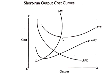
(iv) Short-Run Output Cost Curves

The cost-output relationships can also be shown through the use of graphs. It will be seen that the average fixed cost curve (AFC curve) falls as output rises from lower levels to higher levels. The shape of the average fixed cost curve, therefore, is a rectangular hyperbola.

However, the average variable cost curve (AVC curve) starts rising earlier than the ATC curve. Further, the least cost level of output corresponds to the point LT on the ATC curve and not to the point LV which lies on the AVC curve.

Another important point to be noted is that in Fig. the marginal cost curve (MC curve) intersects both the AVC curve and ATC curve at their minimum points. This is very simple to explain. If marginal cost (MC) is less than the average cost (AC), it will pull AC down. If the MC is greater than AC, it will pull AC up. If the MC is equal to AC, it will neither pull AC up nor down. Hence, MC curve tends to intersect the AC curve at its lowest point.

Similar is the position about the average variable cost curve. It will not make any difference whether MC is going up or down. LT is the lowest point of total cost and LV is the lowest point of variable cost.

The inter-relationships among AVC, ATC, and AFC can be summed up as follows:

  • If both AFC and AVC fall, ATC will also fall.
  • If AFC falls but AVC rises

(a) ATC will fall where the drop in AFC is more than the rise in AVC.

(b) ATC will not fall where the drop in AFC is equal to the rise in AVC.

(c) ATC will rise where the drop in AFC is less than the rise in AVC.

Cost Output Relationship in Long Run

The long run is a period long enough to make all costs variable including such costs as are fixed in the short run. In the short run, variations in output are possible only within the range permitted by the existing fixed plant and equipment. But in the long run, the entrepreneur has before him a number of alternatives which includes the construction of various kinds and sizes of plants.

Thus, there are no fixed costs since the firm has sufficient time to fully adapt its plant. And all costs become variable. In view of this, the long-run costs will refer to the costs of producing different levels of output by changes in the size of plant or scale of production. The long-run cost-output relationship is shown graphically by the long- run cost curve—a curve showing how costs will change when the scale of production is changed.

The concept of long-run costs can be further explained with the help of an illustration. Suppose that at a particular time, a firm operates under average total cost curve U2 and produces OM. Now it is desired to produce ON. If the firm continues under the old scale, its average cost curve will be NT. If the scale of firm is altered, the new cost curve will be U3. The average cost of producing ON will then be NA.

NA is less than NT. So the new scale is preferable to the old one and should be adopted. In the long run, the average cost of producing ON output is NA. This may be called as the long-run cost of producing ON output. It may be noted here that we shall call NA as the long-run cost only so long as the U3 scale is in the planning stage and has not actually been adopted. The moment the scale is installed, the NA cost will be the short-run cost of producing ON output.

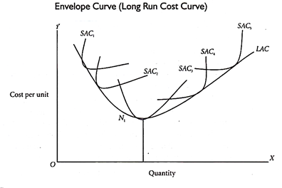
To draw a long-run cost curve, we have to start with a number of short-run average cost curves (SAC curves), each such curve representing a particular scale or size of the plant, including the optimum scale. One can now draw the long-run cost curve which tangential to the entire family of SAC curves, that is, it touches each SAC curve at one point.

error: Content is protected !!