Expansion Path

In economics, an expansion path (also called a scale line) is a curve in a graph with quantities of two inputs, typically physical capital and labor, plotted on the axes. The path connects optimal input combinations as the scale of production expands. A producer seeking to produce a given number of units of a product in the cheapest possible way chooses the point on the expansion path that is also on the isoquant associated with that output level.

Economists Alfred Stonier and Douglas Hague defined “expansion path” as “that line which reflects the least–cost method of producing different levels of output, when factor prices remain constant.” The points on an expansion path occur where the firm’s isocost curves, each showing fixed total input cost, and its isoquants, each showing a particular level of output, are tangent; each tangency point determines the firm’s conditional factor demands. As a producer’s level of output increases, the firm moves from one of these tangency points to the next; the curve joining the tangency points is called the expansion path.

If an expansion path forms a straight line from the origin, the production technology is considered homothetic (or homoethetic). In this case, the ratio of input usages is always the same regardless of the level of output, and the inputs can be expanded proportionately so as to maintain this optimal ratio as the level of output expands. A Cobb–Douglas production function is an example of a production function that has an expansion path which is a straight line through the origin.

Meaning of Expansion Path:

We know that the production function of the firm

q = f(x,y)

Gives us the isoquant map of the firm, one isoquant (IQ) for each particular level of output, and the cost equation of the firm

C = r_Xx + r_Yy           

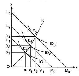
gives us the family of parallel iso-cost lines (ICLs), given the prices of the inputs r_X and r_Y, one ICL for one particular level of cost. The IQ-map and the family of ICLs have been given in Fig. If we now join the point of origin 0 and the points of tangency, E₁, E₂, E₃, etc., between the IQs and the ICLs by a curve, then this curve would give us what is known as the expansion path of the firm.

The expansion path is so called because if the firm decides to expand its operations, it would have to move along this path. Let us note that the firm may expand in two ways.

First, it may want to expand by successively increasing its level of cost or its expenditure on the inputs X and Y, i.e., by using more and more of inputs, and, consequently, by producing more of its output.

Second, the firm may decide to expand by increasing its level of output per period. This the firm may do by increasing the expenditure on the inputs, i.e., by using more and more of them.

The two approaches to expansion apparently appear to be the same, for both involve an increase in expenditure. However, there is a fundamental difference. In the first case, decision is taken initially at the point of cost. Cost levels are made higher and higher and then efforts are made to maximize the level of output subject to the cost constraint.

On the other hand, in the second case, decision-making occurs initially and directly at the point of output. Here the firm first decides to produce more of output and then efforts are made to produce the output at the minimum possible cost.

Types of Expansion Path

1. Expansion by Means of Increasing the Level of Expenditure on the Inputs

In Fig. let us suppose that, initially, the firm’s level of cost is such that its ICL is L₁M₁ and output-maximization subject to cost constraint occurs at the point of tangency, E₁, between the ICL, L₁M₁, and an IQ which is IQ₁. At E₁ the firm uses X₁ of the first input and y₁ of the second input to produce the maximum possible output, say, q₁, which is represented by IQ₁.

Now, if the firm decides to expand by increasing the cost level from the level of L₁M₁ to that of L₂M₂, then the firm would be in output-maximising equilibrium at the point of tangency E₂ (x₂, y₂), on IQ₂, using more of the inputs, x₂ > x₁ and y₂ > y₁, and producing an output level, say, q₂, q₂ > q₁, since IQ₂ is a higher isoquant than IQ₁.

In the same way, if the firm decides to expand further, it would increase its cost level from that of L₂M₂ to that of L₃M₃ and it would produce the maximum output subject to the cost constraint at the point of tangency E₃ (x₃, y₃) on IQ₃ using more of the inputs, x₃ > x₂ and y₃ > y₂, and producing a higher level of output, say, q₃, q₃ > q₂, since IQ₃ is a higher IQ than IQ₂.

The process of expansion of firm’s operations through increases in the level of cost may go on in this say so long as the firm decides in its favour. If we now join the point of origin O and the points E₁, E₂, E₃, etc. by a path, then we would obtain the firm’s expansion path.

That is, if the firm expands by increasing its level of cost, it would have to move successively from one equilibrium point to another along this expansion path.

We have joined the path through the equilibrium points E₁, E₂, etc. with the point of origin O, because if the firm moves backward along the expansion path by decreasing the cost level then it would be moving from the initial equilibrium point, say, E₃ to E₂, then from E₂ to E) and would approach the point O which would be the limiting point in this process.

As the firm’s cost level decreases and tends to zero, the input quantities and the output quantity would all decrease and tend to zero, and thus the point of origin O would be the limiting point.

2. Expansion by Means of Increasing the Level of Output

In Fig. let us suppose that initially the firm decides to produce q₁ of output which can be produced at any point on the isoquant, IQ₁. The firm would be in cost-minimizing equilibrium at the point E₁ which is the point of tangency between IQ₁ and an iso-cost line say, ICL₁. At the point E₁, the firm would use Xi and y] quantities of the two inputs and its cost amounts to, say, C₁, which is the minimum possible.

The firm may now decide to expand by increasing its level of output from q₁ to q₂ on IQ₂. If the firm makes this decision, its cost-minimizing equilibrium will be obtained at the point of tangency E₂ (x₂, y₂) on L₂M₂ using more of the inputs, x₂ > x₁ and y₂ > y₁ and incurring a cost level C₂ on L₂M₂, which is the minimum possible required to produce the output of q₂. However, C₂ > C₁ since L₂M₂ is a higher ICL than L₂M₂.

In the same way, the firm may decide to increase again its level of output from q₂ to q₃ on IQ₃. In this case, the firm’s equilibrium point would be the point of tangency E₃ (x₃, y₃) on the ICL, L₃M₃. At E₃, the firm would use still more of the inputs, x₃ > x₂ and y₃ > y₂, incurring a cost level C₃ on L₃M₃, which is the minimum required for producing q₃ of output. However, C₃ > C₂ since L₃M₃ is a higher ICL than L₂M₂.

The firm’s process of expansion may go on like this as long as it decides to expand. The expansion path again would be OK that would start from the point of origin O and pass through the points E₁, E₂, E₃, etc.

If the firm decides to contract and produce less of output, then the limiting point of the process of contraction would be the point of origin O, where the firm’s use of the inputs, its cost level and output would all tend to zero.

The Equation of the Expansion Path

Each point on the expansion path, is a point of tangency between an isoquant and an iso-cost line. Therefore, at each point on the expansion path, we have numerical slope of the IQ = numerical slope of the ICL

⇒ MRTS_X,Y = r_X/r_Y

⇒ f_X/f_Y= r_X/r_Y = constant [^._.^. r_X and r_Y are given and constant]

Therefore, gives us the equation of the expansion path.