Cost Output Relationship in Short Run and Long Run

Time element plays an important role in price determination of a firm. During short period two types of factors are employed. One is fixed factor while others are variable factors of production. Fixed factor of production remains constant while with the increase in production, we can change variable inputs only because time is short in which all the factors cannot be varied.

Raw material, semi-finished material, unskilled labour, energy, etc., are variable inputs which can be changed during short run. Machines, capital, infrastructure, salaries of managers and technical experts are included in fixed inputs. During short period an individual firm can change variable factors of production according to requirements of production while fixed factors of production cannot be changed.

Cost-Output Relationship in the Short Run

(i) Average Fixed Cost Output

The greater the output, the lesser the fixed cost per unit, i.e., the average fixed cost. The reason is that total fixed costs remain the same and do not change with a change in output.

The relationship between output and fixed cost is a universal one for all types of business.

Thus, average fixed cost falls continuously as output rises. The reason why total fixed costs remain the same and the average fixed cost falls is that certain factors are indivisible. Indivisibility means that if a smaller output is to be produced, the factor cannot be used in a smaller quantity. It is to be used as a whole.

(ii) Average Variable Cost and Output

The average variable costs will first fall and then rise as more and more units are produced in a given plant. This is so because as we add more units of variable factors in a fixed plant, the efficiency of the inputs first increases and then decreases. In fact, the variable factors tend to produce somewhat more efficiently near a firm’s optimum output than at very low levels of output.

But once the optimum capacity is reached, any further increase in output will undoubtedly increase average variable cost quite sharply. Greater output can be obtained but at much greater average variable cost. For example, if more and more workers are appointed. It may ultimately lead to overcrowding and bad organization. Moreover, workers may have to be paid higher wages for overtime work.

(iii) Average Total Cost and Output

Average total costs, more commonly known as average costs, will decline first and then rise upward. The significant point to note here is that the turning point in the case of average cost comes a little later in the case of average variable cost.

Average cost consists of average fixed cost plus average variable cost. As we have seen, average fixed cost continues to fall with an increase in output while average variable cost first declines and then rises. So long as average variable cost declines the average total cost will also decline. But after a point, the average variable cost will rise. Here, if the rise in variable cost is less than the drop in fixed cost, the average total cost will still continue to decline.

It is only when the rise in average variable cost is more than the drop in average fixed cost that the average total cost will show a rise. Thus, there will be a stage where the average variable cost may have started rising yet the average total cost is still declining because the rise in average variable cost is less than the drop in average fixed cost. The net effect being a decline in average cost.

The least cost-output level is the level where the average total cost is the minimum and not the average variable cost. In fact, at the least cost-output level, the average variable cost will be more than its minimum (average variable cost). The least cost- output level is also the optimum output level. It may not be the maximum output level. A firm may decide to produce more than the least cost-output level.

(iv) Short-Run Output Cost Curves

The cost-output relationships can also be shown through the use of graphs. It will be seen that the average fixed cost curve (AFC curve) falls as output rises from lower levels to higher levels. The shape of the average fixed cost curve, therefore, is a rectangular hyperbola.

However, the average variable cost curve (AVC curve) starts rising earlier than the ATC curve. Further, the least cost level of output corresponds to the point LT on the ATC curve and not to the point LV which lies on the AVC curve.

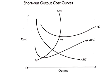
Another important point to be noted is that in Fig. the marginal cost curve (MC curve) intersects both the AVC curve and ATC curve at their minimum points. This is very simple to explain. If marginal cost (MC) is less than the average cost (AC), it will pull AC down. If the MC is greater than AC, it will pull AC up. If the MC is equal to AC, it will neither pull AC up nor down. Hence, MC curve tends to intersect the AC curve at its lowest point.

Similar is the position about the average variable cost curve. It will not make any difference whether MC is going up or down. LT is the lowest point of total cost and LV is the lowest point of variable cost.

The inter-relationships among AVC, ATC, and AFC can be summed up as follows:

• If both AFC and AVC fall, ATC will also fall.
• If AFC falls but AVC rises

(a) ATC will fall where the drop in AFC is more than the rise in AVC.

(b) ATC will not fall where the drop in AFC is equal to the rise in AVC.

(c) ATC will rise where the drop in AFC is less than the rise in AVC.

Cost Output Relationship in Long Run

The long run is a period long enough to make all costs variable including such costs as are fixed in the short run. In the short run, variations in output are possible only within the range permitted by the existing fixed plant and equipment. But in the long run, the entrepreneur has before him a number of alternatives which includes the construction of various kinds and sizes of plants.

Thus, there are no fixed costs since the firm has sufficient time to fully adapt its plant. And all costs become variable. In view of this, the long-run costs will refer to the costs of producing different levels of output by changes in the size of plant or scale of production. The long-run cost-output relationship is shown graphically by the long- run cost curve—a curve showing how costs will change when the scale of production is changed.

The concept of long-run costs can be further explained with the help of an illustration. Suppose that at a particular time, a firm operates under average total cost curve U2 and produces OM. Now it is desired to produce ON. If the firm continues under the old scale, its average cost curve will be NT. If the scale of firm is altered, the new cost curve will be U3. The average cost of producing ON will then be NA.

NA is less than NT. So the new scale is preferable to the old one and should be adopted. In the long run, the average cost of producing ON output is NA. This may be called as the long-run cost of producing ON output. It may be noted here that we shall call NA as the long-run cost only so long as the U3 scale is in the planning stage and has not actually been adopted. The moment the scale is installed, the NA cost will be the short-run cost of producing ON output.

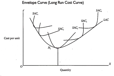
To draw a long-run cost curve, we have to start with a number of short-run average cost curves (SAC curves), each such curve representing a particular scale or size of the plant, including the optimum scale. One can now draw the long-run cost curve which tangential to the entire family of SAC curves, that is, it touches each SAC curve at one point.