 by
by For the analysis of production function with two variable factors we make use of the concept called isoquants or iso-product curves which are similar to indifference curves of the theory of demand. Therefore, before we explain the production function with two variable factors and returns to scale, we shall explain the concept of isoquants (that is, equal product curves) and their properties.
Isoquants
Isoquants, which are also called equal product curves, are similar to the indifference curves of the theory of consumer’s behaviour. An isoquant represents all those factor combinations which are capable of producing the same level of output.
The isoquants are thus contour lines which trace the loci of equal outputs. Since an isoquant represents those combinations of inputs which will be capable of producing an equal quantity of output, the producer would be indifferent between them. Therefore, isoquants are also often called equal product curves production-indifference curves.
Table 1. Factor Combinations to Produce a Given or Level of Output:

The concept of isoquant can be easily understood from Table 1. It is presumed that two factors labour and capital are being employed to produce a product. Each of the factor combinations A. B, C, D and E produces the same level of output, say 100 units. To start with, factor combination A consisting of 1 unit of labour and 12 units of capital produces the given 100 units of output.
Similarly, combination B consisting of 2 units of labour and 8 units of capital, combination C consisting of 3 units of labour and 5 units of capital, combination D consisting of 4 units of labour and 3 units of capital, combination E consisting of 5 units of labour and 2 units of capital are capable of producing the same amount of output, i.e., 100 units. In Fig. 1 we have plotted all these combinations and by joining them we obtain an isoquant showing that every combination represented on it can produce 100 units of output.

Isoquants Though isoquants are similar to be indifference curves of the theory of consumer’s behaviour, there is one important difference between the two. An indifference curve represents all those combinations of two goods which provide the same satisfaction or utility to a consumer but no attempt is made to specify the level of utility in exact quantitative terms it stands for.
This is so because the cardinal measurement of satisfaction or utility in unambiguous thermos is not possible. That is why we usually label indifference curves by ordinal numbers as I, II, III etc. indicating that a higher indifference curve represents a higher level of satisfaction than a lower one, but the information as to how much one level of satisfaction is greater than another is not provided.
On the other hand, we can label isoquants in the physical units of output without any difficulty. Production of a good being a physical phenomenon lends itself easily to absolute measurement in physical units. Since each isoquant represents a specified level of production, it is possible to say by how much one isoquant indicates greater or less production than another.
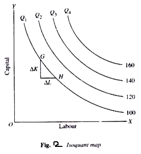
In Fig. 2 we have drawn an isoquant-map or equal- product map with a set of four isoquants which represent 100 units, 120 units, 140 units and 160 units of output respectively. Then, from this set of isoquants it is very easy to judge by how much production level on one isoquant curve is greater or less than on another.
Ridge Lines
The marginal product of a particular factor may be negative if the quantity used is too large. For example, if too much labour is used there may be congestion and the efficiency of all the labourers may be affected. An isoquant will include points denoting such factor quantities, because it includes all factor combinations producing the same output.
But, a rational producer will not operate on this part of the isoquant. The area of rational operation may be shown by drawing two lines from the origin enclosing only those parts of the isoquants where each factor has a positive marginal product. Such lines are called ridge lines. Negative marginal products appear in that part of the isoquant which has a positive slope.
Ridge lines exclude these parts. This can be seen in Fig. 3. Let us focus our attention on isoquant Q1 over the interval from point A to point E. We now know that as we substitute labour for capital and move from A toward E, the marginal productivity of labour diminishes.

But, look what happens if we move beyond E, continuing to use more labour. The isoquant Q1 turns upward, indicating that if we use more labour and still want to produce Q1 units, we must now also use more capital. Why? Because beyond E, the marginal product of labour has become negative, and so to compensate for using more labour, we must add to the amount of capital used as well.
If we follow Q2, Q3 or Q4 from left to right, we see that a similar result occurs. Beyond points F, G and H turn up. That is, the slopes of the isoquants become positive due to the negative marginal productivity of labour.

The line (R’) connecting all points, such as £, F, G and H, is called a ridge line; it marks off the boundary between stage II and stage III of production. No one would want to produce in stage III, since the same level of production could be obtained with fewer of both inputs by moving to the left along the appropriate isoquant until stage II was reached.
We can now apply this same line of reasoning to rule out stage I. Again let us concentrate attention on isoquant Q1. This time, suppose we move up and to the left toward point A. As we do so, substituting capital for labour, the marginal productivity of capital diminishes and becomes negative if we go beyond A. Thus, if we add more capital above A while maintaining output at the Q1 level, we must use more labour.
This does not make much sense from a managerial perspective. Points B, C and D are analogous to point A for their respective isoquants. Beyond these points, the marginal productivity of capital is negative and so we would not wish to operate in that region, which we refer to as stage I.
The ridge line R marks the boundary between stage I and stage II just as R’ marks the boundary between stages II and III. We see that neither stage I nor stage III is desirable for production, since the marginal productivity of at least one input is negative in those stages. We can then conclude that the only relevant region for production is stage II, which is bounded by the two ridge lines, R1 and R2. This region is called the economic region of production.