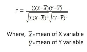
Karl Pearson Coefficient of Correlation (also called the Pearson correlation coefficient or Pearson’s r) is a measure of the strength and direction of the linear relationship between two variables. It ranges from -1 to +1, where +1 indicates a perfect positive linear relationship, -1 indicates a perfect negative linear relationship, and 0 indicates no linear relationship. The formula for Pearson’s r is calculated by dividing the covariance of the two variables by the product of their standard deviations. It is widely used in statistics to analyze the degree of correlation between paired data.
The following are the main properties of correlation.
-
Coefficient of Correlation lies between -1 and +1:
The coefficient of correlation cannot take value less than -1 or more than one +1. Symbolically,
-1<=r<= + 1 or | r | <1.
-
Coefficients of Correlation are independent of Change of Origin:
This property reveals that if we subtract any constant from all the values of X and Y, it will not affect the coefficient of correlation.
-
Coefficients of Correlation possess the property of symmetry:
The degree of relationship between two variables is symmetric as shown below:
-
Coefficient of Correlation is independent of Change of Scale:
This property reveals that if we divide or multiply all the values of X and Y, it will not affect the coefficient of correlation.
- Co-efficient of correlation measures only linear correlation between X and Y.
- If two variables X and Y are independent, coefficient of correlation between them will be zero.
Karl Pearson’s Coefficient of Correlation is widely used mathematical method wherein the numerical expression is used to calculate the degree and direction of the relationship between linear related variables.
Pearson’s method, popularly known as a Pearsonian Coefficient of Correlation, is the most extensively used quantitative methods in practice. The coefficient of correlation is denoted by “r”.
If the relationship between two variables X and Y is to be ascertained, then the following formula is used:
Properties of Coefficient of Correlation
- The value of the coefficient of correlation (r) always lies between±1. Such as:
r=+1, perfect positive correlation
r=-1, perfect negative correlation
r=0, no correlation
- The coefficient of correlation is independent of the origin and scale.By origin, it means subtracting any non-zero constant from the given value of X and Y the vale of “r” remains unchanged. By scale it means, there is no effect on the value of “r” if the value of X and Y is divided or multiplied by any constant.
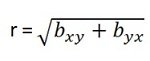
- The coefficient of correlation is a geometric mean of two regression coefficient. Symbolically it is represented as:
- The coefficient of correlation is “ zero” when the variables X and Y are independent. But, however, the converse is not true.
Assumptions of Karl Pearson’s Coefficient of Correlation
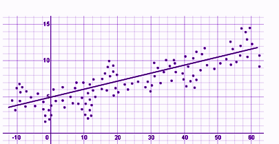
- The relationship between the variables is “Linear”, which means when the two variables are plotted, a straight line is formed by the points plotted.
- There are a large number of independent causes that affect the variables under study so as to form a Normal Distribution. Such as, variables like price, demand, supply, etc. are affected by such factors that the normal distribution is formed.
- The variables are independent of each other.
Note: The coefficient of correlation measures not only the magnitude of correlation but also tells the direction. Such as, r = -0.67, which shows correlation is negative because the sign is “-“ and the magnitude is 0.67.
Spearman Rank Correlation
Spearman rank correlation is a non-parametric test that is used to measure the degree of association between two variables. The Spearman rank correlation test does not carry any assumptions about the distribution of the data and is the appropriate correlation analysis when the variables are measured on a scale that is at least ordinal.
The Spearman correlation between two variables is equal to the Pearson correlation between the rank values of those two variables; while Pearson’s correlation assesses linear relationships, Spearman’s correlation assesses monotonic relationships (whether linear or not). If there are no repeated data values, a perfect Spearman correlation of +1 or −1 occurs when each of the variables is a perfect monotone function of the other.
Intuitively, the Spearman correlation between two variables will be high when observations have a similar (or identical for a correlation of 1) rank (i.e. relative position label of the observations within the variable: 1st, 2nd, 3rd, etc.) between the two variables, and low when observations have a dissimilar (or fully opposed for a correlation of −1) rank between the two variables.
The following formula is used to calculate the Spearman rank correlation:
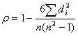
ρ = Spearman rank correlation
di = the difference between the ranks of corresponding variables
n = number of observations
Assumptions
The assumptions of the Spearman correlation are that data must be at least ordinal and the scores on one variable must be monotonically related to the other variable.
Like this:
Like Loading...
 by
by 
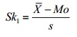
 = the mean, Mo = the mode and s = the standard deviation for the sample.