Tag: Forecasting Methods

Fisher’s Index Number, named after the American economist Irving Fisher, is a composite index that combines elements of both the Laspeyres and Paasche indices to provide a more balanced measure of price changes. It is considered a comprehensive measure because it accounts for both base-period and current-period quantities, offering a more accurate reflection of price changes over time. Here’s an in-depth look at Fisher’s Index Number:

Concept and Purpose:

Fisher’s Index Number aims to address the limitations of the Laspeyres and Paasche indices, which are two commonly used methods for calculating price indices. The Laspeyres Index uses base-period quantities to weigh prices, while the Paasche Index uses current-period quantities. Fisher’s Index blends these approaches to mitigate their individual biases and provide a more accurate measure of price changes.

Calculation

Fisher’s Index Number is calculated as the geometric mean of the Laspeyres Index and the Paasche Index. The formula for Fisher’s Index Number (I_F) is:

I_F= √(L×P)

where:

• L is the Laspeyres Index
• P is the Paasche Index

1. Laspeyres Index

The Laspeyres Index measures the change in price relative to a base period, using base-period quantities for weighting. The formula is:

L = [ ∑(P1×Q0) / ∑(P0×Q0) ]× 100

where:

• P_1 = Price of the item in the current period
• P_0 = Price of the item in the base period
• Q_0 = Quantity of the item in the base period

2. Paasche Index

The Paasche Index measures the change in price relative to a base period, using current-period quantities for weighting. The formula is:

P = [ ∑(P1×Q1) / ∑(P0×Q1) ]× 100

where:

• Q_1 = Quantity of the item in the current period

Steps to Calculate Fisher’s Index

1. Compute the Laspeyres Index: Calculate the price index using base-period quantities to weight current prices.
2. Compute the Paasche Index: Calculate the price index using current-period quantities to weight base prices.
3. Calculate Fisher’s Index: Use the geometric mean of the Laspeyres and Paasche indices.

Applications:

• Comprehensive Price Measurement:

Fisher’s Index provides a balanced approach to measuring price changes by incorporating both base-period and current-period quantities. This makes it a more accurate reflection of real price changes compared to Laspeyres or Paasche indices alone.

• Inflation Analysis:

It is used to assess inflation by comparing changes in the cost of a fixed basket of goods over time, considering variations in both quantity and price.

• Economic Research:

Economists and researchers use Fisher’s Index to study and compare price movements, making it a valuable tool for analyzing trends in economic data.

• Cost of Living Adjustments:

It helps in adjusting wages, salaries, and benefits to keep up with changes in the cost of living by providing a more balanced view of price changes.

Advantages:

• Balanced Measure:

Fisher’s Index avoids the biases inherent in using only base-period or current-period quantities, providing a more balanced view of price changes.

• Accurate Reflection:

It offers a more accurate reflection of price movements by combining the strengths of both the Laspeyres and Paasche indices.

• Geometric Mean:

Using the geometric mean ensures that the index does not overly emphasize one period’s data over another, offering a more neutral perspective.

Limitations:

• Complexity:

Fisher’s Index involves more complex calculations compared to Laspeyres and Paasche indices, which might be less intuitive and more resource-intensive to compute.

• Data Requirements:

It requires detailed data on quantities and prices for accurate computation, which may not always be available.

Un-weighted index numbers are simple index numbers where all items are assigned equal importance or weight, regardless of their actual significance or contribution. These index numbers measure relative changes in prices or quantities without considering the quantity consumed or produced. The Simple Aggregative Method and Simple Average of Price Relatives are commonly used techniques. Though easy to compute and understand, un-weighted index numbers may not accurately reflect real economic scenarios because they ignore the actual impact of each item. Therefore, they are mainly used for illustrative or preliminary analysis rather than precise economic measurement.

Properties of Un-weighted Index Numbers:

• Equal Importance to All Items

Un-weighted index numbers treat all items in the dataset with equal importance, regardless of their actual usage, cost, or impact. This means a low-cost or rarely used item influences the index as much as a high-cost or frequently used item. While this simplifies calculations, it can distort the true picture of economic trends. This property limits the accuracy of un-weighted indices in reflecting real-life consumption or production patterns.

• Simplicity in Calculation

Un-weighted index numbers are easy to compute because they do not require additional data like weights or quantities. Only the prices or quantities from the base and current periods are needed. This simplicity makes them ideal for quick estimates or introductory statistical analysis. However, this ease comes at the cost of precision and relevance, especially when different items have significantly varied importance or impact in the real-world context.

• Distorted Representativeness

Because they assign equal weight to all items, un-weighted index numbers may give a distorted representation of overall price or quantity changes. For instance, a major change in a high-volume product could be overshadowed by minor changes in several low-impact items. This lack of representativeness means that un-weighted indices can mislead policymakers or businesses if used for serious economic or financial decision-making.

• Limited Real-World Application

Due to their disregard for item importance, un-weighted index numbers have limited use in actual business or economic analysis. They are mostly used for academic or theoretical purposes, such as teaching basic statistical concepts. In practical scenarios like inflation tracking or market analysis, weighted index numbers are preferred as they offer a more realistic and reliable measure of change based on actual consumption, sales, or production data.

Types of Un-weighted Index Numbers:

• Simple Aggregative Index Number

This method calculates the index by summing the current period prices and dividing them by the sum of base period prices, multiplied by 100. The formula is:

Simple Aggregative Index = (∑P1 / ∑P0) × 100

Where P1​ and P0​ are current and base period prices. All items are treated equally, regardless of their significance. While easy to compute, it can be misleading if high-priced items disproportionately affect the result. It is suitable for basic analysis but lacks real-world precision.

• Simple Average of Price Relatives Index

This method calculates the price relative for each item (current price divided by base price × 100) and then takes the arithmetic mean of all these relatives. Formula:

Simple Average of Price Relatives = [∑(P1 / P0×100)] / n​

Where $n$ is the number of items. This approach ensures each item has equal influence on the final index, regardless of actual importance. It’s more refined than the aggregative method and reduces the impact of extreme values, but still does not reflect real consumption patterns or weights.

Variation refers to the differences or fluctuations in data values within a dataset. In business, understanding variation is essential for making informed decisions, as it helps identify patterns, trends, and inconsistencies in processes or outcomes. Variation can be natural (random) or assignable (caused by specific factors). It occurs in areas like production, sales, customer behavior, and financial metrics. By measuring variation using statistical tools (like range, variance, and standard deviation), businesses can improve quality control, forecast demand, and reduce risks. Effective analysis of variation supports better resource allocation and strategic planning in uncertain environments.

Properties of Variation:

• Non-Negativity

Variation is always non-negative, meaning its value cannot be less than zero. A variation of zero indicates that all data values are identical, showing no spread. This property ensures that variation is a reliable measure of data dispersion. Since squared differences are used in calculations like variance or standard deviation, negative values are mathematically eliminated, reinforcing consistency in representing the extent of data fluctuations.

• Basis for Dispersion

Variation serves as the foundation for measuring dispersion in data. It quantifies how much individual values deviate from the mean or central value. Higher variation indicates that data points are widely spread out, while lower variation implies closeness to the average. This helps in comparing datasets and assessing consistency, reliability, and control in business processes and decision-making scenarios like quality control or performance monitoring.

• Dependence on Data Scale

Variation is scale-dependent, meaning its value is influenced by the units of the data. For example, the variation in centimeters will differ from the same data measured in meters. This property makes direct comparisons across datasets difficult unless standardized. In such cases, coefficient of variation is used to eliminate the unit-based effect and allow fair comparison between different data groups or scales.

• Influence of Extreme Values

Variation is sensitive to outliers or extreme values. A single unusually high or low value can significantly increase the variation, especially in measures like variance and standard deviation. This sensitivity helps in identifying potential anomalies or quality issues in business processes, but it also means that variation must be interpreted carefully, especially in datasets where extreme values may distort the overall view.

• Used for Comparative Analysis

Variation allows comparison of consistency between two or more datasets. For example, two production machines might produce the same average output, but one may have a higher variation, indicating less reliability. By analyzing variation, managers can choose better-performing systems or predict future outcomes more effectively. It plays a vital role in fields such as finance, marketing, operations, and quality assurance.

Skewness

Skewness is a statistical measure that describes the asymmetry or deviation from symmetry in a distribution of data. When a dataset is perfectly symmetrical, it has zero skewness. If the data tails more towards the right (positive skew), it indicates that a majority of values are concentrated on the lower end. Conversely, a left tail (negative skew) shows values concentrated on the higher end. Skewness helps in understanding the shape of the data distribution, which is important for choosing appropriate statistical methods, interpreting trends, and making informed business decisions based on non-normal or irregular data patterns.

Properties of Skewness:

• Direction of Asymmetry

Skewness indicates the direction in which data deviates from symmetry. If the skewness is positive, the tail on the right side of the distribution is longer, indicating more lower values. If it’s negative, the left tail is longer, indicating more higher values. This property helps understand how data is spread around the mean.

• Impact on Mean and Median

In a skewed distribution, the mean, median, and mode are not equal. In positively skewed data, the mean > median > mode. In negatively skewed data, the mean < median < mode. This helps identify the nature of the distribution and is crucial when selecting the right measure of central tendency for analysis.

• Quantitative Measure

Skewness is measured using formulas like Pearson’s or Bowley’s coefficient of skewness. These give numerical values where zero represents symmetry, positive values indicate right skew, and negative values indicate left skew. This numerical property allows easy comparison between datasets and helps assess how far a distribution deviates from normality.

• Unitless Value

Skewness is a dimensionless (unitless) number, meaning it is unaffected by the units of the variable being measured. This allows comparisons of skewness between different datasets, regardless of their scales or units. It also makes skewness a standardized measure, helping in interpreting data shapes across various domains and applications.

• Sensitivity to Outliers

Skewness is highly sensitive to outliers because extreme values in the data can significantly pull the tail, altering the skewness value. A few large or small values can make an otherwise symmetric distribution appear skewed. This property makes skewness useful in detecting outliers and data irregularities during statistical analysis.

Key differences between Variation and Skewness

Significance of Measuring Variation:

• Improves Decision Making

Measuring variation helps managers understand the reliability and stability of data. By identifying how much values deviate from the average, decision-makers can assess risks and choose better strategies. For instance, in sales forecasting, recognizing variation in customer demand allows for better inventory planning. Quantifying variation also helps differentiate between normal fluctuations and unusual patterns, leading to more data-driven, informed decisions that align with business goals.

• Enhances Quality Control

In production and service processes, measuring variation is crucial for maintaining consistent quality. It helps identify deviations from standards and detect defects or process inefficiencies. Tools like control charts and standard deviation enable businesses to monitor performance, reduce errors, and maintain customer satisfaction. By minimizing unnecessary variation, companies can achieve higher quality outputs, reduce costs, and ensure compliance with regulatory or industry standards.

• Enables Process Improvement

Variation measurement is a foundation for continuous improvement initiatives such as Six Sigma or Total Quality Management. It allows organizations to pinpoint sources of inconsistency and implement targeted improvements. By reducing unwanted variation, businesses can make operations more efficient, predictable, and cost-effective. Over time, this leads to streamlined workflows, reduced waste, and enhanced productivity, giving companies a competitive edge in both manufacturing and service sectors.

• Assists in Risk Management

Understanding variation helps identify uncertainties and potential risks in business processes. By analyzing variation in financial performance, customer behavior, or supply chain reliability, managers can develop strategies to mitigate risks. For example, consistent variation in supplier delivery times may require contingency planning. Measuring variation allows firms to prepare for worst-case scenarios, allocate resources wisely, and build resilience against market volatility or operational disruptions.

Properties of Good Variation:

• Predictability

Good variation exhibits a consistent and predictable pattern over time. This predictability allows businesses to make reliable forecasts and informed decisions. For example, seasonal sales patterns or daily website traffic variations help managers plan inventory, staffing, or marketing strategies effectively. Predictable variation supports stability in processes, enabling smoother operations and better planning for future trends or demand changes.

• Relevance

A good variation is relevant to the business objective or decision-making process. It should provide meaningful insights that help identify opportunities or problems. For instance, analyzing variation in customer preferences can guide product development. Irrelevant variations, on the other hand, may distract decision-makers. Focusing on relevant variations ensures that the analysis is purpose-driven and aligned with organizational goals, helping managers focus on impactful factors.

• Measurability

Good variation must be quantifiable using statistical methods such as mean, standard deviation, or variance. Measurability ensures that the variation can be analyzed, tracked over time, and compared across different datasets. For example, tracking the variation in daily production output helps monitor consistency. Without measurability, it becomes difficult to evaluate performance or identify areas for improvement, limiting the effectiveness of quantitative analysis.

• Consistency

Good variation maintains a consistent pattern under similar conditions. If the variation changes erratically without any identifiable cause, it may indicate underlying problems. Consistency in variation allows businesses to establish control limits and set performance benchmarks. In manufacturing, for example, consistent variation in product quality indicates a stable process, while inconsistent variation may point to equipment or human error.

• Informative Value

Good variation provides insights that lead to better decision-making. It should reveal underlying trends, root causes, or patterns that support corrective actions or strategy formulation. For instance, variation in customer complaints across regions can highlight service issues. An informative variation goes beyond raw data and contributes to knowledge generation, making it a valuable input in business intelligence and strategic analysis.

• Controllability

Good variation should be capable of being monitored and controlled to a reasonable extent. If a variation can be managed through process improvement, training, or better systems, it becomes useful for continuous improvement. For example, reducing variation in delivery time improves customer satisfaction. Controllability transforms variation into an opportunity for operational excellence and efficiency, aligning with total quality management principles.

Simple Average or Price Relatives Method

In this method, we find out the price relative of individual items and average out the individual values. Price relative refers to the percentage ratio of the value of a variable in the current year to its value in the year chosen as the base.

Price relative (R) = (P1÷P2) × 100

Here, P1= Current year value of item with respect to the variable and P2= Base year value of the item with respect to the variable. Effectively, the formula for index number according to this method is:

 P = ∑[(P1÷P2) × 100] ÷N

Here, N= Number of goods and P= Index number.

Weighted index method

Weighted Aggregate Method

Here different goods are assigned weight according to the quantity bought. There are three well-known sub-methods based on the different views of economists as mentioned below:

Laspeyre’s Method

Laspeyre was of the view that base year quantities must be chosen as weights. Therefore the formula is :

P = (∑P₁Q₀÷∑P₀Q₀)×100

Here,  ∑P₁Q₀= Summation of prices of current year multiplied by quantities of the base year taken as weights and ∑P₀Q₀= Summation of, prices of base year multiplied by quantities of the base year taken as weights.

Paasche Index Number

The Paasche Price Index is a consumer price index used to measure the change in the price and quantity of a basket of goods and services relative to a base year price and observation year quantity. Developed by German economist Hermann Paasche, the Paasche Price Index is commonly referred to as the “current weighted index.”

Formula for the Paasche Price Index

The formula for the index is as follows:

Where:

• Pi,0 is the price of the individual item at the base period and Pi,t is the price of the individual item at the observation period.
• Qi,t is the quantity of the individual item at the observation period.

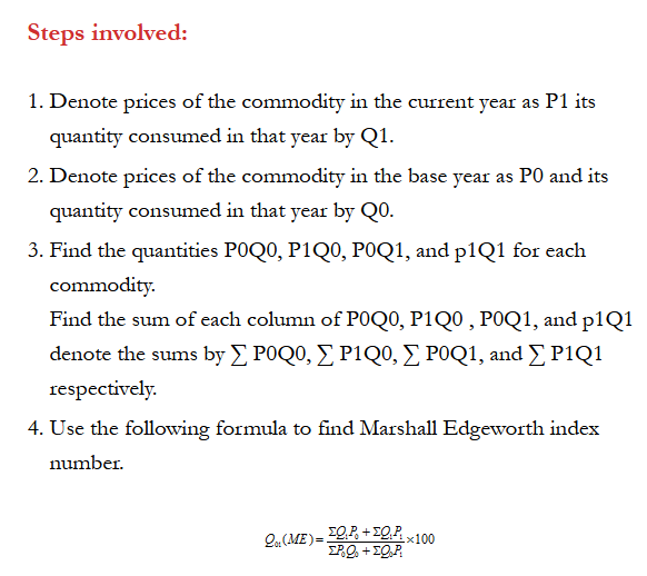
Marshall Edgeworth Index Number

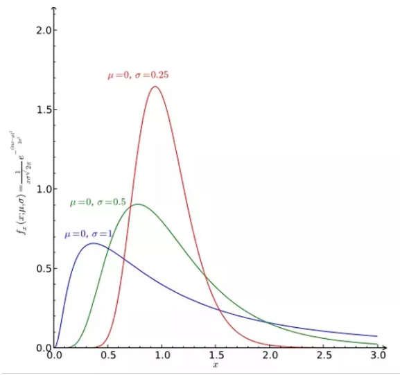
Skewness, in statistics, is the degree of distortion from the symmetrical bell curve, or normal distribution, in a set of data. Skewness can be negative, positive, zero or undefined. A normal distribution has a skew of zero, while a lognormal distribution, for example, would exhibit some degree of right-skew.

The three probability distributions depicted below depict increasing levels of right (or positive) skewness. Distributions can also be left (negative) skewed. Skewness is used along with kurtosis to better judge the likelihood of events falling in the tails of a probability distribution.

Right skewness

• Skewness, in statistics, is the degree of distortion from the symmetrical bell curve in a probability distribution.
• Distributions can exhibit right (positive) skewness or left (negative) skewness to varying degree.
• Investors note skewness when judging a return distribution because it, like kurtosis, considers the extremes of the data set rather than focusing solely on the average.

Broadly speaking, there are two types of skewness: They are

(1) Positive skewness

(2) Negative skewnes.

Positive skewness

A series is said to have positive skewness when the following characteristics are noticed:

• Mean > Median > Mode.
• The right tail of the curve is longer than its left tail, when the data are plotted through a histogram, or a frequency polygon.
• The formula of Skewness and its coefficient give positive figures.

Negative Skewness

A series is said to have negative skewness when the following characteristics are noticed:

• Mode> Median > Mode.
• The left tail of the curve is longer than the right tail, when the data are plotted through a histogram, or a frequency polygon.
• The formula of skewness and its coefficient give negative figures.

Thus, a statistical distribution may be three types viz.

• Symmetric
• Positively skewed
• Negatively skewed

Skewness Co-efficient

1. Pearson’s Coefficient of Skewness #1 uses the mode. The formula is:

   

   Where  = the mean, Mo = the mode and s = the standard deviation for the sample.

2. Pearson’s Coefficient of Skewness #2 uses the median. The formula is:

   

   Where  = the mean, Mo = the mode and s = the standard deviation for the sample.

   It is generally used when you don’t know the mode.