Median (Calculation and graphical using ogives)

The median of a set of data values is the middle value of the data set when it has been arranged in ascending order.  That is, from the smallest value to the highest value.

Example:

The marks of nine students in a geography test that had a maximum possible mark of 50 are given below:

47

35

37

32

38

39

36

34

35

Find the median of this set of data values.

Solution:

Arrange the data values in order from the lowest value to the highest value:

32

34

35

35

36

37

38

39

47

The fifth data value, 36, is the middle value in this arrangement.

Merits or Uses of Median:

1. Median is rigidly defined as in the case of Mean.
2. Even if the value of extreme item is much different from other values, it is not much affected by these values e.g. Median in case of 4, 7, 12, 18, 19 is 12 and if we add two values equal to 450 10000, new median is 18.
3. It can also be used for the Quantities; those can’t give A.M; as is in case of intelligence etc. It is possible to arrange in any order and to locate the middle valve. For such cases it is the best measure.
4. It can be located graphically.
5. For open end intervals, it is also suitable one. As taking any value of the intervals, value of Median remains the same.
6. It can be easily calculated and is also easy to understand
7. Median is also used for other statistical devices such as Mean Deviation and skewness.
8. It can be located by inspection in some cases.
9. Extreme items may not be available to get Median. Only if number of terms is known, we can get median e.g.

Find median of the 9 terms, out of which first two and last three terms are missing and middle four terms are 7, 9, 10, 14. Here we can calculate as following let nine terms be

*

*

7

9

10

14

*

*

*

Here out of nine terms middle term is; (n+1/2) Thus 10 is the Median.

Demerits or Limitations of Median:

1. Even if the value of extreme items is too large, it does not affect too much, but due to this reason, sometimes median does not remain the representative of the series.
2. It is affected much more by fluctuations of sampling than A.M.
3. Median cannot be used for further algebraic treatment. Unlike mean we can neither find total of terms as in case of A.M. nor median of some groups when combined.
4. In a continuous series it has to be interpolated. We can find its true-value only if the frequencies are uniformly spread over the whole class interval in which median lies.
5. If the number of series is even, we can only make its estimate; as the A.M. of two middle terms is taken as Median.

Graphical Method

Marks	Conversion into exclusive series	No. of students	Cumulative Frequency
(x)		(f)	(C.M)
410-419	409.5-419.5	14	14
420-429	419.5-429.5	20	34
430-439	429.5-439.5	42	76
440-449	439.5-449.5	54	130
450-459	449.5-459.5	45	175
460-469	459.5-469.5	18	193
470-479	469.5-479.5	7	200

The median value of a series may be determinded through the graphic presentation of data in the form of Ogives.This can be done in 2 ways.

1. Presenting the data graphically in the form of ‘less than’ ogive or ‘more than’ ogive .
   2. Presenting the data graphically and simultaneously in the form of ‘less than’ and ‘more than’ ogives.The two ogives are drawn together.
2. Less than Ogive approach

Marks	Cumulative Frequency (C.M)
Less than 419.5	14
Less than 429.5	34
Less than 439.5	76
Less than 449.5	130
Less than 459.5	175
Less than 469.5	193
Less than 479.5	200

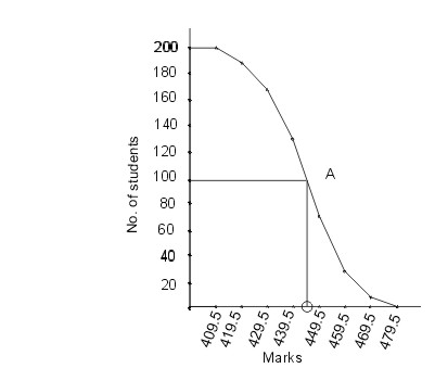
Steps involved in calculating median using less than Ogive approach:
1. Convert the series into a ‘less than ‘ cumulative frequency distribution as shown above.

2. Let N be the total number of students who’s data is given.N will also be the cumulative frequency of the last interval.Find the (N/2)^th item(student) and mark it on the y-axis.In this case the (N/2)^th item (student) is 200/2 = 100^th student.
3. Draw a perpendicular from 100 to the right to cut the Ogive curve at point A.
4. From point A where the Ogive curve is cut, draw a perpendicular on the x-axis. The point at which it touches the x-axis will be the median value of the series as shown in the graph.

More than Ogive approach

Marks	Cumulative Frequency (C.M)
More than 409.5	200
More than 419.5	186
More than 429.5	166
More than 439.5	124
More than 449.5	70
More than 459.5	25
More than 469.5	7
More than 479.5	0

Steps involved in calculating median using more than Ogive approach:
1. Convert the series into a ‘more than ‘ cumulative frequency distribution as shown above .
2. Let N be the total number of students who’s data is given.N will also be the cumulative frequency of the last interval.Find the (N/2)^th item(student) and mark it on the y-axis.In this case the (N/2)^th item (student) is 200/2 = 100^th student.
3. Draw a perpendicular from 100 to the right to cut the Ogive curve at point A.
4.From point A where the Ogive curve is cut, draw a perpendicular on the x-axis. The point at which it touches the x-axis will be the median value of the series as shown in the graph.

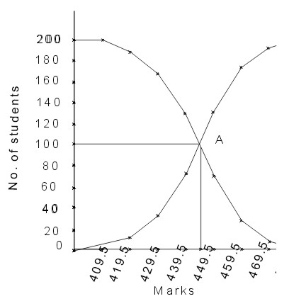
2. Less than and more than Ogive approach

Another way of graphical determination of median is through simultaneous graphic presentation of both the less than and more than Ogives.

1.Mark the point A where the Ogive curves cut each other.
2.Draw a perpendicular from A on the x-axis. The corresponding value on the x-axis would be the median value.