Break Even Point: Meaning, Features and Significance

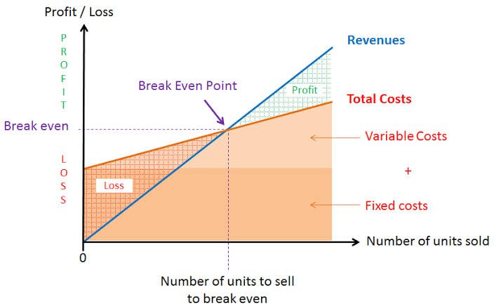
Break-even point represents that volume of production where total costs equal to total sales revenue resulting into a no-profit no-loss situation.

In simple words, the break-even point can be defined as a point where total costs (expenses) and total sales (revenue) are equal. Break-even point can be described as a point where there is no net profit or loss. The firm just “breaks even.” Any company which wants to make abnormal profit, desires to have a break-even point. Graphically, it is the point where the total cost and the total revenue curves meet.

Calculation (formula)

Break-even point is the number of units (N) produced which make zero profit.

Revenue – Total costs = 0

Total costs = Variable costs * N + Fixed costs

Revenue = Price per unit * N

Price per unit * N – (Variable costs * N + Fixed costs) = 0

So, break-even point (N) is equal

N = Fixed costs / (Price per unit – Variable costs)

About Break-even point

The origins of break-even point can be found in the economic concepts of “the point of indifference.” Calculating the break-even point of a company has proved to be a simple but quantitative tool for the managers. The break-even analysis, in its simplest form, facilitates an insight into the fact about revenue from a product or service incorporates the ability to cover the relevant production cost of that particular product or service or not. Moreover, the break-even point is also helpful to managers as the provided info can be used in making important decisions in business, for example preparing competitive bids, setting prices, and applying for loans.

Adding more to the point, break-even analysis is a simple tool defining the lowest quantity of sales which will include both variable and fixed costs. Moreover, such analysis facilitates the managers with a quantity which can be used to evaluate the future demand. If, in case, the break-even point lies above the estimated demand, reflecting a loss on the product, the manager can use this info for taking various decisions. He might choose to discontinue the product, or improve the advertising strategies, or even re-price the product to increase demand.

Another important usage of the break-even point is that it is helpful in recognizing the relevance of fixed and variable cost. The fixed cost is less with a more flexible personnel and equipment thereby resulting in a lower break-even point. The importance of break-even point, therefore, cannot be overstated for a sound business and decision making.

However, the applicability of break-even analysis is affected by numerous assumptions. A violation of these assumptions might result in erroneous conclusions.

Features of Break Even Point

(i) It helps in the determination of selling price which will give the desired profits.

(ii) It helps in the fixation of sales volume to cover a given return on capital employed.

(iii) It helps in forecasting costs and profit as a result of change in volume.

(iv) It gives suggestions for shift in sales mix.

(v) It helps in making inter-firm comparison of profitability.

(vi) It helps in determination of costs and revenue at various levels of output.

(vii) It is an aid in management decision-making (e.g., make or buy, introducing a product etc.), forecasting, long-term planning and maintaining profitability.

(viii) It reveals business strength and profit earning capacity of a concern without much difficulty and effort.

Significance of Break Even Point

(i) All costs can be separated into fixed and variable components

(ii) Fixed costs will remain constant at all volumes of output

(iii) Variable costs will fluctuate in direct proportion to volume of output

(iv) Selling price will remain constant

(v) Product-mix will remain unchanged

(vi) The number of units of sales will coincide with the units produced so that there is no opening or closing stock

(vii) Productivity per worker will remain unchanged

(viii) There will be no change in the general price level

Limitations of Break-Even Analysis

  1. Break-even analysis is based on the assumption that all costs and expenses can be clearly separated into fixed and variable components. In practice, however, it may not be possible to achieve a clear-cut division of costs into fixed and variable types.
  2. It assumes that fixed costs remain constant at all levels of activity. It should be noted that fixed costs tend to vary beyond a certain level of activity.
  3. It assumes that variable costs vary proportionately with the volume of output. In practice, they move, no doubt, in sympathy with volume of output, but not necessarily in direct proportions..
  4. The assumption that selling price remains unchanged gives a straight revenue line which may not be true. Selling price of a product depends upon certain factors like market demand and supply, competition etc., so it, too, hardly remains constant.
  5. The assumption that only one product is produced or that product mix will remain unchanged is difficult to find in practice.
  6. Apportionment of fixed cost over a variety of products poses a problem.
  7. It assumes that the business conditions may not change which is not true.
  8. It assumes that production and sales quantities are equal and there will be no change in opening and closing stock of finished product, these do not hold good in practice.
  9. The break-even analysis does not take into consideration the amount of capital employed in the business. In fact, capital employed is an important determinant of the profitability of a concern.

Cost: Output Relationship in Short and Long Run

Cost Output Relationship in Short Run

Time element plays an important role in price determination of a firm. During short period two types of factors are employed. One is fixed factor while others are variable factors of production. Fixed factor of production remains constant while with the increase in production, we can change variable inputs only because time is short in which all the factors cannot be varied.

Raw material, semi-finished material, unskilled labour, energy, etc., are variable inputs which can be changed during short run. Machines, capital, infrastructure, salaries of managers and technical experts are included in fixed inputs. During short period an individual firm can change variable factors of production according to requirements of production while fixed factors of production cannot be changed.

Cost-Output Relationship in the Short Run:

(i) Average Fixed Cost Output

The greater the output, the lesser the fixed cost per unit, i.e., the average fixed cost. The reason is that total fixed costs remain the same and do not change with a change in output.

The relationship between output and fixed cost is a universal one for all types of business.

Thus, average fixed cost falls continuously as output rises. The reason why total fixed costs remain the same and the average fixed cost falls is that certain factors are indivisible. Indivisibility means that if a smaller output is to be produced, the factor cannot be used in a smaller quantity. It is to be used as a whole.

(ii) Average Variable Cost and Output

The average variable costs will first fall and then rise as more and more units are produced in a given plant. This is so because as we add more units of variable factors in a fixed plant, the efficiency of the inputs first increases and then decreases. In fact, the variable factors tend to produce somewhat more efficiently near a firm’s optimum output than at very low levels of output.

But once the optimum capacity is reached, any further increase in output will undoubtedly increase average variable cost quite sharply. Greater output can be obtained but at much greater average variable cost. For example, if more and more workers are appointed. It may ultimately lead to overcrowding and bad organization. Moreover, workers may have to be paid higher wages for overtime work.

(iii) Average Total Cost and Output

Average total costs, more commonly known as average costs, will decline first and then rise upward. The significant point to note here is that the turning point in the case of average cost comes a little later in the case of average variable cost.

Average cost consists of average fixed cost plus average variable cost. As we have seen, average fixed cost continues to fall with an increase in output while average variable cost first declines and then rises. So long as average variable cost declines the average total cost will also decline. But after a point, the average variable cost will rise. Here, if the rise in variable cost is less than the drop in fixed cost, the average total cost will still continue to decline.

It is only when the rise in average variable cost is more than the drop in average fixed cost that the average total cost will show a rise. Thus, there will be a stage where the average variable cost may have started rising yet the average total cost is still declining because the rise in average variable cost is less than the drop in average fixed cost. The net effect being a decline in average cost.

The least cost-output level is the level where the average total cost is the minimum and not the average variable cost. In fact, at the least cost-output level, the average variable cost will be more than its minimum (average variable cost). The least cost- output level is also the optimum output level. It may not be the maximum output level. A firm may decide to produce more than the least cost-output level.

(iv) Short-Run Output Cost Curves

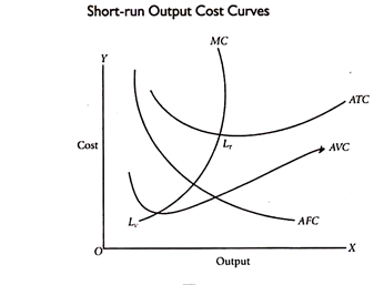
The cost-output relationships can also be shown through the use of graphs. It will be seen that the average fixed cost curve (AFC curve) falls as output rises from lower levels to higher levels. The shape of the average fixed cost curve, therefore, is a rectangular hyperbola.

However, the average variable cost curve (AVC curve) starts rising earlier than the ATC curve. Further, the least cost level of output corresponds to the point LT on the ATC curve and not to the point LV which lies on the AVC curve.

Another important point to be noted is that in Fig. the marginal cost curve (MC curve) intersects both the AVC curve and ATC curve at their minimum points. This is very simple to explain. If marginal cost (MC) is less than the average cost (AC), it will pull AC down. If the MC is greater than AC, it will pull AC up. If the MC is equal to AC, it will neither pull AC up nor down. Hence, MC curve tends to intersect the AC curve at its lowest point.

Similar is the position about the average variable cost curve. It will not make any difference whether MC is going up or down. LT is the lowest point of total cost and LV is the lowest point of variable cost.

The inter-relationships among AVC, ATC, and AFC can be summed up as follows:

  • If both AFC and AVC fall, ATC will also fall.
  • If AFC falls but AVC rises

(a) ATC will fall where the drop in AFC is more than the rise in AVC.

(b) ATC will not fall where the drop in AFC is equal to the rise in AVC.

(c) ATC will rise where the drop in AFC is less than the rise in AVC.

Cost Output Relationship in Long Run

The long run is a period long enough to make all costs variable including such costs as are fixed in the short run. In the short run, variations in output are possible only within the range permitted by the existing fixed plant and equipment. But in the long run, the entrepreneur has before him a number of alternatives which includes the construction of various kinds and sizes of plants.

Thus, there are no fixed costs since the firm has sufficient time to fully adapt its plant. And all costs become variable. In view of this, the long-run costs will refer to the costs of producing different levels of output by changes in the size of plant or scale of production. The long-run cost-output relationship is shown graphically by the long- run cost curve—a curve showing how costs will change when the scale of production is changed.

The concept of long-run costs can be further explained with the help of an illustration. Suppose that at a particular time, a firm operates under average total cost curve U2 and produces OM. Now it is desired to produce ON. If the firm continues under the old scale, its average cost curve will be NT. If the scale of firm is altered, the new cost curve will be U3. The average cost of producing ON will then be NA.

NA is less than NT. So the new scale is preferable to the old one and should be adopted. In the long run, the average cost of producing ON output is NA. This may be called as the long-run cost of producing ON output. It may be noted here that we shall call NA as the long-run cost only so long as the U3 scale is in the planning stage and has not actually been adopted. The moment the scale is installed, the NA cost will be the short-run cost of producing ON output.

To draw a long-run cost curve, we have to start with a number of short-run average cost curves (SAC curves), each such curve representing a particular scale or size of the plant, including the optimum scale. One can now draw the long-run cost curve which tangential to the entire family of SAC curves, that is, it touches each SAC curve at one point.

Cost Concepts Meaning and Types of Costs

According to the Chartered Institute of Management Accountants, cost is “the amount of expenditure (actual or notional) incurred on or attributable to a specified thing or activity.” Similarly, according to Anthony and Wilsch “cost is a measurement in monetary terms of the amount of resources used for some purposes.”

Cost has been defined by the Committee on Cost Terminology of the American Accounting Association as “the foregoing, in monetary terms, incurred or potentially to be incurred in the realization of the objective of management which may be manufacturing of a product or rendering of a service.”

From the above, it may be stated that cost means the total of all expenses incurred for a product or a service. Thus, cost of an article means the actual outgoings or ascertained changes incurred in its production and sale activities. In short, it is the amount of resources used up in exchange for some goods or services.

The so-called resources are expressed in terms of money or monetary units. What we stated above will not be a meaningful one until the same is used with an adjective only, i.e. when it communicates the meaning for which it is intended.

Thus, when we say Prime Cost or Works Cost or Fixed Cost etc., we want to explain a particular meaning which is essential while computing, measuring or analyzing the various aspects of cost.

Classification of Cost

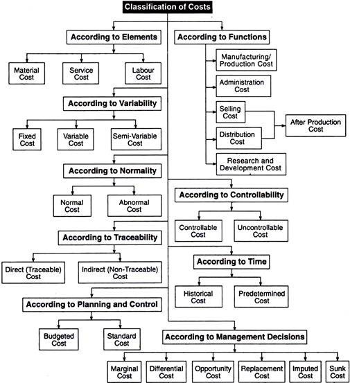
Classification of costs implies the process of grouping costs according to their common characteristics. A proper classification of costs is absolutely necessary to mention the costs with cost centres. Usually, costs are classified according to their nature, viz., material, labour, over-head, among others. An identical cost figure may be classified in various ways according to the needs of the firms.

The above classification may be outlined as:

The classification of cost may be depicted as given:

  1. According to Elements

Under the circumstances, costs are classified into three broad categories Material, Labour and Overhead. Now, further subdivision may also be made for each of them. For example, Material may be subdivided into raw materials, packing materials, consumable stores etc. This classification is very useful in order to ascertain the total cost and its components. Same classification may also be made for labour and overhead.

  1. According to Functions

The total costs are divided into different segments according to the purpose of the firm. That is why costs are grouped as per the requirements of the firm in order to evaluate its functions properly. In short, the total costs include all costs starting from cost of materials to the cost of packing the product.

It takes the cost of direct material, direct labour and chargeable expenses and all indirect expenses under the head Manufacturing/Production cost.

At the same time, administration cost (i.e. relating to office and administration) and Selling and Distribution expenses (i.e. relating to sales) are to be classified separately and to be added in order to find out the total cost of the product. If these functional classifications are not made properly, true cost of the product cannot accurately be ascertained.

  1. According to Variability

Practically, costs are classified according to their behaviour relating to the change (increase or decrease) in their volume of activity.

These costs as per volume may be subdivided into:

(i) Fixed Cost

(ii) Variable Cost

(iii) Semi-variable Cost

Fixed Costs are those which do not vary with the change in output, i.e., irrespective of the quantity of output produced, it remains fixed (e.g., Salaries, Rent etc.) up to a certain limit. It is interesting to note that if more units are product, fixed cost per unit will be reduced, and, if less units are produced, obviously, fixed cost per unit will be increased.

Variable Costs, on the other hand, are those which vary proportionately with the volume of output. So the cost per unit will remain fixed irrespective of the quantity produced. That is, there is no direct effect on the cost per unit if there is a change in the volume of output (e.g. price of raw material, labour etc.,).

On the contrary, semi-variable costs are those which are partly fixed and partly variable (e.g. Repairs of building).

  1. According to Controllability

Costs may, again, be subdivided into two broad categories according to the performance done by any member of the firm.

They are:

(i) Controllable Costs; and

(ii) Uncontrollable Costs.

Controllable Costs are those costs which may be influenced by the decision taken by a specified member of the administration of the firm or, it may be stated, that the costs which at least partly depend on the management and is controllable by them, e.g. all direct costs, direct material, direct labour and chargeable expenses (components of Prime Cost) are controllable by lower management level and is done accordingly.

Uncontrollable Costs are those which are not influenced by the actions taken by any specific member of the management. For example, fixed costs, viz., rent of building, payment for salaries etc.

  1. According to Normality

Under this condition, costs are classified according to the normal needs for a given level of output for a normal level of activity produced for such output.

They are divided into:

(i) Normal Costs

(ii) Abnormal Costs

Normal Costs are those costs which are normally required for a normal production at a given level of output and which is a part of production.

Abnormal Costs, on the other hand, are those costs which are not normally required for a given level of output to be produced normally, or which is not a part of cost of production.

  1. According to Time

Costs may also be classified according to the time element in it. Accordingly, costs are classified into:

(i) Historical Costs

(ii) Predetermined Costs.

Historical Costs are those costs which are taken into consideration after they have been incurred. This is possible particularly when the production of a particular unit of output has already been made. They have only historical value and cannot assist in controlling costs.

Predetermined Costs, on the other hand, are the estimated costs. Such costs are computed in advanced on the basis of past experience and records. Needless to say here that it becomes standard cost if it is determined on scientific basis. When such standard costs are compared with the actual costs, the reasons of variance will come out which will help the management to take proper steps for reconciliation.

  1. According to Traceability

Costs can be identified with a particular product, process, department etc. They are divided into:

(i) Direct (Traceable) Costs

(ii) Indirect (Non-Traceable) Costs.

Direct/Traceable Costs are those costs which can directly be traced or allocated to a product, i.e. it includes all traceable costs, viz., all expenses relating to cost of raw materials, labour and other service utilised which can be traced easily.

Indirect/Non-Traceable Costs are those costs which cannot directly be traced or allocated to a product, i.e. it includes all non-traceable costs, e.g. salary of store-keepers, general administrative expenses, i.e. which cannot properly be allocated directly to a product.

  1. According to Planning and Control

Costs may also be classified into:

(i) Budgeted Costs

(ii) Standard Costs.

Budgeted Costs refer to the expected cost of manufacture computed on the basis of information available in advance of actual production or purchase. Practically, budgeted costs include standard costs, both are predetermined costs and their amount may coincide but their objectives are different.

Standard Costs, on the other hand, is a predetermination of what actual costs should be under projected conditions serving as a basis of cost control and, as a measure of product efficiency, when ultimately aligned actual cost. It supplies a medium by which the effectiveness of current results can be measured and the responsibility for derivations can be placed.

Standard Costs are predetermined for each element, viz., material, labour and overhead.

Standard Costs include

(i) The cost per unit is determined to make an estimated total output for the future period for:

(a) Material

(b) Labour

(c) Overhead.

(ii) The cost must depend on the past experience and experiments and specification of the technical staff.

(iii) The cost must be expressed in terms of rupees.

  1. According to Management Decisions

Under this, costs may also be classified as:

(a) Marginal Cost: Marginal Cost is the cost for producing additional unit or units by segregation of fixed costs (i.e., cost of capacity) from variable cost (i.e. cost of production) which helps to know the profitability. Moreover, we know, in order to increase the production, certain expenses (fixed) may not increase at all, only some expenses relating to materials, labour and variable expenses are increased. Thus, the total cost so increased by the production of one unit or more is the cost of marginal unit and the cost is known as marginal cost or incremental cost.

(b) Differential Cost: Differential Cost is that portion of the cost of a function attributable to and identifiable with an added feature, i.e. the change in costs as a result of change in the level of activity or method of production.

(c) Opportunity Cost: It is the prospective change in cost following the adoption of an alternative machine, process, raw materials, specification or operation. In other words, it is the maximum possible alternative earnings which might have been earned if the existing capacity had been changed to some other alternative way.

(d) Replacement Cost: It is the cost, at current prices, in a particular locality or market area, of replacing an item of property or a group of assets.

(e) Implied Cost: It is the cost used to indicate the presence of arbitrary or subjective elements of product cost having more than usual significance. It is also called notional cost, e.g., interest on capital although no interest is paid. This is particularly useful while decisions are taken regarding alternative capital investment projects.

(f) Sunk Cost: It is the past cost arising out of a decision which cannot be revised now, and associated with specialised equipment’s or other facilities not readily adaptable to present or future purposes. Such cost is often regarded as constituting a minor factor in decisions affecting the future.

Iso-Product Curves- Meaning and Features

An iso-product curve is locus of various combinations of two factors of production giving the same level of output and a producer is indifferent to each of such combinations. All the combinations of two inputs give the same quantum of output to a producer and the producer is indifferent to each such combination. He does not have any preference. These iso-product curves are also called production indifference curves. The concept of iso-product curve can be explained with the help of iso-quant schedule and diagram.

Assumptions:

The main assumptions of Iso-quant curves are as follows:

  1. Two Factors of Production:

Only two factors are used to produce a commodity.

  1. Divisible Factor:

Factors of production can be divided into small parts.

  1. Constant Technique:

Technique of production is constant or is known beforehand.

  1. Possibility of Technical Substitution:

The substitution between the two factors is technically possible. That is, production function is of ‘variable proportion’ type rather than fixed proportion.

  1. Efficient Combinations:

Under the given technique, factors of production can be used with maximum efficiency.

Iso-Quant Schedule

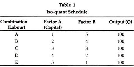
An iso-quant schedule shows different combinations of two factors of production (inputs) at which a producer gets equal quantum of output.

The schedule is given below:

The above schedule shows the different combinations of two inputs, namely, labour and capital and the resultant output 100 units from each combination. The units of labour are increasing and units of capital are decreasing but the quantity of output remains the same.

The schedule can be depicted in the form of a diagram given below:

In the diagram factor A and factor B are shown on OX-axis and OY-axis respectively. IP is the iso-product curve showing the different combinations (A, B, C, D and E) of the two factors of production giving the same quantity of output (100 units).

The IP curve slopes downward to the right. It explains with the increase in the units of factor-A when we are reducing the units of factor-B.

Iso-Product Curve and Indifference Curve

The shape and slope of iso-product curve and indifference curve are similar but both of them have the following differences:

(1) Iso-product curve shows the quantum of output while an indifference curve shows the level of satisfaction. Iso-product curve shows the different combinations of two factors of production (inputs) showing the same quantum of output but an indifference curve shows the different combinations of two commodities showing the same level of satisfaction.

(2) We can prepare an iso-product map by which we can express that how much less or more quantity of output is shown by each iso-product curve but an indifference curve cannot say how much more or less is the satisfaction from different combinations of two commodities a consumer is getting. Utility or satisfaction is not measurable but the quantity of output is measurable with the help of iso-product curve.

Features of Iso-Product Curves

The following are the characteristics of iso-product curves:

(1) Iso-Product Curves Slope Downward to the Right

Iso- product curves slope downward to the right because producer has limited resources with alternative uses and he is faced with the problem of choice. He cannot increase the amount of labour and capital. If he employs more of labour he has to employ less of capital in order to get the same level of output as given in the following diagram:

The diagram shows that units of labour are shown on OX- axis and units of capital on OY-axis. A combination shows OK of capital and OL of labour while at B combination OK1 of capital and OL1 of labour showing the same amount of output (100 units). But the producer has employed more of labour and less of capital and on account of it the iso-product curve slopes downward to the right.

(2) Iso-Product Curves are Convex to the Origin

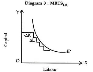
As an indifference curve is convex to the origin, similarly an iso-product curve is also convex to the origin. In an iso-product curve a factor of production is substituted by another factor of production and consequently the marginal rate of technical substitution of labour for capital (MRTSLK) declines and on account of decreasing MRTSLK the iso-product curves are convex to the origin.

It is shown by the following diagram:

The table reveals that we are increasing the units of labour and reducing the units of capital. The MRTSLK shows a declining trend.

(3) Two Iso-Product Curve never Intersect Each Other

Another characteristic is that two iso-product curves do not intersect each other as different iso-product curves show different level of output.

It is shown by the following diagram:

Capital and labour are shown on OY-axis and OX-axis respectively. IP and IPX are two iso-product curves. E is the point where IP2 and IP1 intersect each other.

Before E point IP1 is higher than IP2 and after E point IP1 is higher than IP. In such a situation it is difficult to know which Iso- product curve gives higher level of output. Hence, we can say that it is indeterminate and two iso-product curves do not cut each other.

(4) Higher the Iso-Quant Curve Higher is the Level of Output

A producer gets the same level of output with different combinations of two inputs on the iso-product curve. But in case of different iso-product curves the level of output differs. Higher the iso-product curve, higher the level of output and lower the iso-product, lower will be the level of output. It can be seen from Diagram 5.

The diagram shows Iso-product map in which three Iso- product curves are showing different levels of output. IP, IP1 and IP2 are showing 500 units, 1000 units and 1500 units respectively which show increasing trends. Higher the iso-product curve higher is the level of output (IP to IP2), lower the iso-product curve lower will be the level of output (IP2 to IP). The highest iso-product curve is IP2 and the lowest iso-product curve is IP.

(5) No Isoquant can Touch Either Axis:

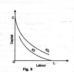
If an isoquant touches X-axis, it would mean that the product is being produced with the help of labour alone without using capital at all. These logical absurdities for OL units of labour alone are unable to produce anything. Similarly, OC units of capital alone cannot produce anything without the use of labour. Therefore as seen in figure 9, IQ and IQ1 cannot be isoquants.

(6) Each Isoquant is Oval-Shaped.

It means that at some point it begins to recede from each axis. This shape is a consequence of the fact that if a producer uses more of capital or more of labour or more of both than is necessary, the total product will eventually decline. The firm will produce only in those segments of the isoquants which are convex to the origin and lie between the ridge lines. This is the economic region of production. In Figure 10, oval shaped isoquants are shown.

Curves OA and OB are the ridge lines and in between them only feasible units of capital and labour can be employed to produce 100, 200, 300 and 400 units of the product. For example, OT units of labour and ST units of the capital can produce 100 units of the product, but the same output can be obtained by using the same quantity of labour T and less quantity of capital VT.

Thus only an unwise entrepreneur will produce in the dotted region of the iso-quant 100. The dotted segments of an isoquant are the waste- bearing segments. They form the uneconomic regions of production. In the up dotted portion, more capital and in the lower dotted portion more labour than necessary is employed. Hence GH, JK, LM, and NP segments of the elliptical curves are the isoquants.

Marginal Rate of Technical Substitution (MRTS)

Marginal rate of technical substitution is an important concept in the study of iso-product curve analysis.

The marginal rate of technical substitution is the rate at which two factors of production (inputs) are substituted. For example, we have two factors of production—capital and labour. The marginal rate of technical substitution of labour for capital (MRTSLK) is that rate at which one unit of labour substitutes the number of units of capital.

The MRTSLK can be studied from the following table:

The table reveals that all the combinations of factor A (labour) and factor B (capital) give the same level of output. If he has C combination then 1A+12B will give the same level of output when he employs 5 units of A and 2 units of B (5A+2B) at G combination the level of output remains unchanged. Hence, the marginal rate of technical substitution of factor A for factor B can be written mathematically in the following formula:

MRTSab = ΔB/ΔA

Thus the MRTSAB shows the marginal rate of technical substitution of A factor for B factor.

Generally, the MRTS declines because as we employ more of factor A then we have to employ less of factor B. It is called the MRTS and each iso-product is conveyed to origin on account of declining MRTS.

Iso-Cost Curve

Different combinations of two inputs give the same level of output which is shown by an iso-product curve. Higher the iso-product curve higher will be the level of output. A producer is faced with the problem of choice because his resources are limited and they have alternative uses.

The choice of a producer depends upon the resources at his disposal and the factor prices. An iso-cost curve shows the various combinations of two inputs (labour and capital) that can be employed by a producer with his given resources. It means the resources of a producer and price of two inputs are shown by this curve. It is given in the Diagram 6.

The diagram shows labour and capital on OX-axis and OY- axis respectively. AB, A1B1 and A2B2 are iso-cost line or curves showing different combinations of labour and capital. If the producer wants to employ more of labour and capital then he should keep in his mind his budget and the prices of both these factors. Higher the iso-cost curve higher will be the need for resources. Iso-cost curve is also known as outlay line, input price line and factor cost 

Returns to scale

“The term returns to scale refers to the changes in output as all factors change by the same proportion.” – Koutsoyiannis

“Returns to scale relates to the behaviour of total output as all inputs are varied and is a long run concept”.  Leibhafsky

It is important to realize that the study of production completely differs according to the time frame. Recollect that we take the help of the law of diminishing returns to study production in the short run, whereas in the long run, the returns to scale are at the helm.

Again, the long run is a long enough period in which we can alter both fixed and variable factors. Thus, in the long run, we aim to study the effect of the changes in all the inputs on the production output.

However, these changes are not random. All the factors are increased or decreased together. This is also known as changes in scale, hence the name return to scale.

Thus, in the long run, we proportionately vary the inputs and observe the relative change in production. Of course, the return to scale can be of three types- increasing, decreasing and constant

Returns to scale are of the following three types

  1. Increasing Returns to scale.
  2. Constant Returns to Scale
  3. Diminishing Returns to Scale

In the long run, output can be increased by increasing all factors in the same proportion. Generally, laws of returns to scale refer to an increase in output due to increase in all factors in the same proportion. Such an increase is called returns to scale.

Suppose, initially production function is as follows:

P = f (L, K)

Now, if both the factors of production i.e., labour and capital are increased in same proportion i.e., x, product function will be rewritten as.

The above stated table explains the following three stages of returns to scale:

  1. Increasing Returns to Scale

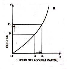
Increasing returns to scale or diminishing cost refers to a situation when all factors of production are increased, output increases at a higher rate. It means if all inputs are doubled, output will also increase at the faster rate than double. Hence, it is said to be increasing returns to scale. This increase is due to many reasons like division external economies of scale. Increasing returns to scale can be illustrated with the help of a diagram 8.

In this figure , OX axis represents increase in labour and capital while OY axis shows increase in output. When labour and capital increases from Q to Q1, output also increases from P to P1 which is higher than the factors of production i.e. labour and capital.

  1. Diminishing Returns to Scale

Diminishing returns or increasing costs refer to that production situation, where if all the factors of production are increased in a given proportion, output increases in a smaller proportion. It means, if inputs are doubled, output will be less than doubled. If 20 percent increase in labour and capital is followed by 10 percent increase in output, then it is an instance of diminishing returns to scale.

The main cause of the operation of diminishing returns to scale is that internal and external economies are less than internal and external diseconomies. It is clear from diagram 9.

In this diagram, diminishing returns to scale has been shown. On OX axis, labour and capital are given while on OY axis, output. When factors of production increase from Q to Q1 (more quantity) but as a result increase in output, i.e. P to P1 is less. We see that increase in factors of production is more and increase in production is comparatively less, thus diminishing returns to scale apply.

  1. Constant Returns to Scale

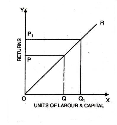
Constant returns to scale or constant cost refers to the production situation in which output increases exactly in the same proportion in which factors of production are increased. In simple terms, if factors of production are doubled output will also be doubled.

In this case internal and external economies are exactly equal to internal and external diseconomies. This situation arises when after reaching a certain level of production, economies of scale are balanced by diseconomies of scale. This is known as homogeneous production function. Cobb-Douglas linear homogenous production function is a good example of this kind. This is shown in diagram. In figure, we see that increase in factors of production i.e. labour and capital are equal to the proportion of output increase. Therefore, the result is constant returns to scale.

CONSTANT RETURNS TO SCALE

For constant returns to scale to occur, the relative change in production should be equal to the proportionate change in the factors.

For example, if all the factors are proportionately doubled, then constant returns would imply that the production output would also double. Interestingly, the production function of an economy as a whole exhibits close characteristics of constant returns to scale.

Also, studies suggest that an individual firm passes through a long phase of constant return to scale in its lifetime. Lastly, it is also known as the linear homogeneous production function.

INCREASING RETURNS TO SCALE

Here, the proportionate increase in production is greater than the increase in inputs. Note that upon expansion, a firm experiences increasing returns to scale. The indivisibility of factors is another reason for this.

Some factors are available in large units, such that they are completely suitable for large-scale production. Evidently, if all the factors are perfectly divisible then there might be no increasing returns. Further, specialization of land and machinery can be another reason.

DECREASING RETURNS TO SCALE

An incidence of decreasing returns to scale would mean that the increase in output is less than the proportionate increase in the input. Generally, this happens when a firm expands all its inputs, especially a large firm.

When the firm expands to a very large size, it becomes difficult to manage it with the same efficiency as before. Hence, the increasing complexity in management, coordination, and control eventually leads to decreasing returns.

Cobb Douglas Production Function

The Cobb Douglas production function {Q(L, K)=A(L^b)K^a}exhibits the three types of returns:

  • If a+b>1, there are increasing returns to scale.
  • For a+b=1, we get constant returns to scale.
  • If a+b<1, we get decreasing returns to scale.

Law of variable Proportions: Definition, Assumption, Graphical Presentation and Stages of the Law

Law of Variable Proportions occupies an important place in economic theory. This law is also known as Law of Proportionality.

Keeping other factors fixed, the law explains the production function with one factor variable. In the short run when output of a commodity is sought to be increased, the law of variable proportions comes into operation.

Therefore, when the number of one factor is increased or decreased, while other factors are constant, the proportion between the factors is altered. For instance, there are two factors of production viz., land and labour.

Land is a fixed factor whereas labour is a variable factor. Now, suppose we have a land measuring 5 hectares. We grow wheat on it with the help of variable factor i.e., labour. Accordingly, the proportion between land and labour will be 1: 5. If the number of laborers is increased to 2, the new proportion between labour and land will be 2: 5. Due to change in the proportion of factors there will also emerge a change in total output at different rates. This tendency in the theory of production called the Law of Variable Proportion.

“As the proportion of the factor in a combination of factors is increased after a point, first the marginal and then the average product of that factor will diminish.” Benham

“An increase in some inputs relative to other fixed inputs will in a given state of technology cause output to increase, but after a point the extra output resulting from the same additions of extra inputs will become less and less.” Samuelson

“The law of variable proportion states that if the inputs of one resource is increased by equal increment per unit of time while the inputs of other resources are held constant, total output will increase, but beyond some point the resulting output increases will become smaller and smaller.” Leftwitch

Assumption of Law of variable Proportions

Law of variable proportions is based on following assumptions:

(i) Constant Technology

The state of technology is assumed to be given and constant. If there is an improvement in technology the production function will move upward.

(ii) Factor Proportions are Variable

The law assumes that factor proportions are variable. If factors of production are to be combined in a fixed proportion, the law has no validity.

(iii) Homogeneous Factor Units

The units of variable factor are homogeneous. Each unit is identical in quality and amount with every other unit.

(iv) Short-Run

The law operates in the short-run when it is not possible to vary all factor inputs.

Graphic Presentation

In fig. 1, on OX axis, we have measured number of labourers while quantity of product is shown on OY axis. TP is total product curve. Up to point ‘E’, total product is increasing at increasing rate. Between points E and G it is increasing at the decreasing rate. Here marginal product has started falling. At point ‘G’ i.e., when 7 units of labourers are employed, total product is maximum while, marginal product is zero. Thereafter, it begins to diminish corresponding to negative marginal product. In the lower part of the figure MP is marginal product curve.

Up to point ‘H’ marginal product increases. At point ‘H’, i.e., when 3 units of labourers are employed, it is maximum. After that, marginal product begins to decrease. Before point ‘I’ marginal product becomes zero at point C and it turns negative. AP curve represents average product. Before point ‘I’, average product is less than marginal product. At point ‘I’ average product is maximum. Up to point T, average product increases but after that it starts to diminish.

Three Stages of the Law

  1. First Stage

First stage starts from point ‘O’ and ends up to point F. At point F average product is maximum and is equal to marginal product. In this stage, total product increases initially at increasing rate up to point E. between ‘E’ and ‘F’ it increases at diminishing rate. Similarly marginal product also increases initially and reaches its maximum at point ‘H’. Later on, it begins to diminish and becomes equal to average product at point T. In this stage, marginal product exceeds average product (MP > AP).

  1. Second Stage

It begins from the point F. In this stage, total product increases at diminishing rate and is at its maximum at point ‘G’ correspondingly marginal product diminishes rapidly and becomes ‘zero’ at point ‘C’. Average product is maximum at point ‘I’ and thereafter it begins to decrease. In this stage, marginal product is less than average product (MP < AP).

  1. Third Stage

This stage begins beyond point ‘G’. Here total product starts diminishing. Average product also declines. Marginal product turns negative. Law of diminishing returns firmly manifests itself. In this stage, no firm will produce anything. This happens because marginal product of the labour becomes negative. The employer will suffer losses by employing more units of labourers. However, of the three stages, a firm will like to produce up to any given point in the second stage only.

In Which Stage Rational Decision is Possible

To make the things simple, let us suppose that, a is variable factor and b is the fixed factor. And a1, a2 , a3….are units of a and b1 b2b3…… are unit of b.

Stage I is characterized by increasing AP, so that the total product must also be increasing. This means that the efficiency of the variable factor of production is increasing i.e., output per unit of a is increasing. The efficiency of b, the fixed factor, is also increasing, since the total product with b1 is increasing.

The stage II is characterized by decreasing AP and a decreasing MP, but with MP not negative. Thus, the efficiency of the variable factor is falling, while the efficiency of b, the fixed factor, is increasing, since the TP with b1 continues to increase.

Finally, stage III is characterized by falling AP and MP, and further by negative MP. Thus, the efficiency of both the fixed and variable factor is decreasing.

Rational Decision

Stage II becomes the relevant and important stage of production. Production will not take place in either of the other two stages. It means production will not take place in stage III and stage I. Thus, a rational producer will operate in stage II.

Suppose b were a free resource; i.e., it commanded no price. An entrepreneur would want to achieve the greatest efficiency possible from the factor for which he is paying, i.e., from factor a. Thus, he would want to produce where AP is maximum or at the boundary between stage I and II.

If on the other hand, a were the free resource, then he would want to employ b to its most efficient point; this is the boundary between stage II and III.

Obviously, if both resources commanded a price, he would produce somewhere in stage II. At what place in this stage production takes place would depend upon the relative prices of a and b.

Condition or Causes of Applicability

There are many causes which are responsible for the application of the law of variable proportions.

  1. Under Utilization of Fixed Factor

In initial stage of production, fixed factors of production like land or machine, is under-utilized. More units of variable factor, like labour, are needed for its proper utilization. As a result of employment of additional units of variable factors there is proper utilization of fixed factor. In short, increasing returns to a factor begins to manifest itself in the first stage.

  1. Fixed Factors of Production

The foremost cause of the operation of this law is that some of the factors of production are fixed during the short period. When the fixed factor is used with variable factor, then its ratio compared to variable factor falls. Production is the result of the co-operation of all factors. When an additional unit of a variable factor has to produce with the help of relatively fixed factor, then the marginal return of variable factor begins to decline.

  1. Optimum Production

After making the optimum use of a fixed factor, then the marginal return of such variable factor begins to diminish. The simple reason is that after the optimum use, the ratio of fixed and variable factors become defective. Let us suppose a machine is a fixed factor of production. It is put to optimum use when 4 labourers are employed on it. If 5 labourers are put on it, then total production increases very little and the marginal product diminishes.

  1. Imperfect Substitutes

Mrs. Joan Robinson has put the argument that imperfect substitution of factors is mainly responsible for the operation of the law of diminishing returns. One factor cannot be used in place of the other factor. After optimum use of fixed factors, variable factors are increased and the amount of fixed factor could be increased by its substitutes.

Such a substitution would increase the production in the same proportion as earlier. But in real practice factors are imperfect substitutes. However, after the optimum use of a fixed factor, it cannot be substituted by another factor.

Applicability of the Law of Variable Proportions

The law of variable proportions is universal as it applies to all fields of production. This law applies to any field of production where some factors are fixed and others are variable. That is why it is called the law of universal application.

The main cause of application of this law is the fixity of any one factor. Land, mines, fisheries, and house building etc. are not the only examples of fixed factors. Machines, raw materials may also become fixed in the short period. Therefore, this law holds good in all activities of production etc. agriculture, mining, manufacturing industries.

  1. Application to Agriculture

With a view of raising agricultural production, labour and capital can be increased to any extent but not the land, being fixed factor. Thus when more and more units of variable factors like labour and capital are applied to a fixed factor then their marginal product starts to diminish and this law becomes operative.

  1. Application to Industries

In order to increase production of manufactured goods, factors of production has to be increased. It can be increased as desired for a long period, being variable factors. Thus, law of increasing returns operates in industries for a long period. But, this situation arises when additional units of labour, capital and enterprise are of inferior quality or are available at higher cost.

As a result, after a point, marginal product increases less proportionately than increase in the units of labour and capital. In this way, the law is equally valid in industries.

Postponement of the Law

The postponement of the law of variable proportions is possible under following conditions:

(i) Improvement in Technique of Production

The operation of the law can be postponed in case variable factors techniques of production are improved.

(ii) Perfect Substitute

The law of variable proportion can also be postponed in case factors of production are made perfect substitutes i.e., when one factor can be substituted for the other.

Production, Meaning, Factors of Production, Production Function, Features, Types

Production is a fundamental economic activity that involves transforming inputs into outputs to satisfy human wants and needs. It refers to the creation of utility by converting raw materials, natural resources, and various inputs such as labor and capital into finished goods or services. The term “production” is not confined only to manufacturing physical products but also includes the provision of services like healthcare, education, transportation, and banking.

In economics, production is defined as any activity that results in the generation of value. It adds utility in terms of form (changing the shape or structure of goods), place (making goods available where they are needed), and time (making goods available when they are required). For instance, converting cotton into fabric or providing consultancy services both fall under the scope of production.

Production plays a central role in the functioning of any economy. It is the backbone of economic development, as it creates goods and services, generates income, provides employment, and contributes to the GDP. The process involves the effective combination and utilization of the four factors of production—land, labor, capital, and entrepreneurship.

Efficient production ensures cost-effectiveness, quality output, and customer satisfaction. In a competitive business environment, firms continuously seek to improve their production processes through innovation and technology. Thus, production is not merely a technical activity but also a strategic function that directly influences business performance and market success.

Factors of Production:

  • Land

Land refers to all natural resources used in the creation of goods and services. This includes physical land, forests, minerals, water, and other gifts of nature. It is a passive factor but essential, as it provides the base for agriculture, manufacturing, and infrastructure. The availability and productivity of land influence industrial location and output. It is fixed in supply and subject to diminishing returns if overused without improvement or technological intervention.

  • Labour

Labor represents the human effort—both physical and mental—used in production. It includes the work of employees, professionals, and skilled or unskilled workers. The productivity of labor depends on education, health, skills, motivation, and working conditions. Labor is an active factor that contributes directly to the creation of goods and services. Effective labor management and training programs can enhance output, efficiency, and innovation, making labor a critical resource in competitive business environments.

  • Capital

Capital comprises man-made resources such as tools, machinery, buildings, and technology used to produce other goods and services. It differs from money, as capital refers specifically to physical assets that facilitate production. Capital improves labor productivity and production efficiency. It can be categorized into fixed capital (long-term assets) and working capital (short-term inputs). Businesses must invest in and maintain capital assets to scale operations and stay technologically competitive in dynamic markets.

  • Entrepreneurship

Entrepreneurship is the ability to identify opportunities, organize resources, take risks, and innovate. Entrepreneurs combine land, labor, and capital to initiate and manage production activities. They are the decision-makers who determine what, how, and for whom to produce. Successful entrepreneurs drive innovation, generate employment, and stimulate economic growth. Their risk-taking ability and vision are essential for launching new ventures and sustaining businesses in a changing economic landscape.

  • Human Capital

Human capital refers to the knowledge, skills, experience, and competencies possessed by individuals. Unlike labor, which measures effort, human capital emphasizes quality and expertise. Investment in education, training, and healthcare improves human capital, leading to higher productivity and innovation. In knowledge-driven economies, human capital is crucial for sectors like IT, R&D, and services. Businesses that cultivate strong human capital gain a strategic advantage through creativity, efficiency, and decision-making capabilities.

  • Information and Knowledge

Information and knowledge have become key production factors in the digital era. Access to market data, consumer insights, and industry trends enables firms to make informed decisions and respond to changes swiftly. Knowledge fuels innovation, strategy, and process improvement. Companies use data analytics and research to optimize supply chains, target customers, and reduce risks. In the modern economy, intangible assets like intellectual property and brand reputation also derive from valuable information.

  • Time

Time, though often overlooked, is a vital factor of production. It affects productivity, cost-efficiency, and market responsiveness. Timely decision-making, project execution, and delivery influence customer satisfaction and profitability. Time also determines the depreciation of assets and the lifecycle of products. Efficient time management leads to leaner operations and better resource utilization. In fast-moving markets, the ability to act quickly on opportunities is a decisive competitive advantage.

  • Technology

Technology enhances all other factors of production by increasing efficiency, reducing costs, and enabling innovation. It transforms traditional processes into automated, scalable, and intelligent systems. For instance, AI, robotics, and cloud computing streamline manufacturing, logistics, and customer service. Technology reduces reliance on physical labor and optimizes capital usage. In modern business strategy, adopting and upgrading technology is not optional—it is essential for survival, growth, and staying ahead in competitive markets.

Production Function:

Production Function is an economic concept that describes the relationship between the inputs used in production and the resulting output. It shows how different combinations of labor, capital, and other factors of production contribute to the production of goods or services. The production function helps in understanding the efficiency of resource utilization, and how changes in the quantity of inputs affect the level of output. It is often expressed as an equation or graph, representing the technological relationship in production.

Mathematically, such a basic relationship between inputs and outputs may be expressed as:

Q = f( L, C, N )

Where

Q = Quantity of output

L = Labour

C = Capital

N = Land.

Hence, the level of output (Q), depends on the quantities of different inputs (L, C, N) available to the firm. In the simplest case, where there are only two inputs, labour (L) and capital (C) and one output (Q), the production function becomes.

Q = f(L, C)

“The production function is a technical or engineering relation between input and output. As long as the natural laws of technology remain unchanged, the production function remains unchanged.” Prof. L.R. Klein

“Production function is the relationship between inputs of productive services per unit of time and outputs of product per unit of time.” Prof. George J. Stigler

“The relationship between inputs and outputs is summarized in what is called the production function. This is a technological relation showing for a given state of technological knowledge how much can be produced with given amounts of inputs.” Prof. Richard J. Lipsey

Thus, from the above definitions, we can conclude that production function shows for a given state of technological knowledge, the relation between physical quantities of inputs and outputs achieved per period of time.

Features of Production Function:

Following are the main features of production function:

1. Substitutability

The factors of production or inputs are substitutes of one another which make it possible to vary the total output by changing the quantity of one or a few inputs, while the quantities of all other inputs are held constant. It is the substitutability of the factors of production that gives rise to the laws of variable proportions.

2. Complementarity

The factors of production are also complementary to one another, that is, the two or more inputs are to be used together as nothing will be produced if the quantity of either of the inputs used in the production process is zero.

The principles of returns to scale is another manifestation of complementarity of inputs as it reveals that the quantity of all inputs are to be increased simultaneously in order to attain a higher scale of total output.

3. Specificity

It reveals that the inputs are specific to the production of a particular product. Machines and equipment’s, specialized workers and raw materials are a few examples of the specificity of factors of production. The specificity may not be complete as factors may be used for production of other commodities too. This reveals that in the production process none of the factors can be ignored and in some cases ignorance to even slightest extent is not possible if the factors are perfectly specific.

Production involves time; hence, the way the inputs are combined is determined to a large extent by the time period under consideration. The greater the time period, the greater the freedom the producer has to vary the quantities of various inputs used in the production process.

In the production function, variation in total output by varying the quantities of all inputs is possible only in the long run whereas the variation in total output by varying the quantity of single input may be possible even in the short run.

Time Period and Production Functions

The production function is differently defined in the short run and in the long run. This distinction is extremely relevant in microeconomics. The distinction is based on the nature of factor inputs.

Those inputs that vary directly with the output are called variable factors. These are the factors that can be changed. Variable factors exist in both, the short run and the long run. Examples of variable factors include daily-wage labour, raw materials, etc.

On the other hand, those factors that cannot be varied or changed as the output changes are called fixed factors. These factors are normally characteristic of the short run or short period of time only. Fixed factors do not exist in the long run.

Consequently, we can define two production functions: short-run and long-run. The short-run production function defines the relationship between one variable factor (keeping all other factors fixed) and the output. The law of returns to a factor explains such a production function.

For example, consider that a firm has 20 units of labour and 6 acres of land and it initially uses one unit of labour only (variable factor) on its land (fixed factor). So, the land-labour ratio is 6:1. Now, if the firm chooses to employ 2 units of labour, then the land-labour ratio becomes 3:1 (6:2).

The long-run production function is different in concept from the short run production function. Here, all factors are varied in the same proportion. The law that is used to explain this is called the law of returns to scale. It measures by how much proportion the output changes when inputs are changed proportionately.

Types of Production Function:

1. Short-Run Production Function

In the short run, at least one input is fixed (usually capital), while other inputs (like labor) are variable. The short-run production function examines how changes in variable inputs affect output, keeping the fixed input constant.

Key Features:

  • Focuses on the law of variable proportions (diminishing marginal returns).
  • Output increases initially at an increasing rate, then at a decreasing rate, and eventually may decline.

Example:

A factory with fixed machinery (capital) adds more workers (labor). Initially, productivity increases, but as workers crowd the factory, additional output diminishes.

2. Long-Run Production Function

In the long run, all inputs are variable, allowing firms to adjust labor, capital, and other resources fully. The long-run production function focuses on the optimal combination of inputs to achieve maximum efficiency and output.

Key Features:

  • Examines returns to scale:
    • Increasing Returns to Scale: Doubling inputs results in more than double the output.
    • Constant Returns to Scale: Doubling inputs results in a proportional doubling of output.
    • Decreasing Returns to Scale: Doubling inputs results in less than double the output.
  • Useful for long-term planning and investment decisions.

3. Cobb-Douglas Production Function

A mathematical representation of the relationship between two or more inputs (e.g., labor and capital) and output. It is commonly expressed as:

Q = A*L^α*K^β*

Where:

  • Q: Total output
  • L: Labor input
  • K: Capital input
  • α,β: Elasticities of output with respect to labor and capital
  • A: Total factor productivity

Key Features:

  • Demonstrates the contribution of labor and capital to output.
  • Widely used in economics for empirical studies and forecasting.

4. Fixed Proportions Production Function (Leontief Production Function)

In this type, inputs are used in fixed proportions to produce output. Increasing one input without proportionately increasing the other does not lead to higher output.

Example:

A car requires one engine and four tires. Adding more engines without increasing the number of tires will not produce more cars.

5. Variable Proportions Production Function

Inputs can be substituted for one another in varying proportions while producing the same level of output.

Example:

A firm can use either more machines and less labor or more labor and fewer machines to produce the same output.

6. Isoquant Production Function

An isoquant represents all possible combinations of two inputs (e.g., labor and capital) that produce the same level of output. The isoquant approach analyzes how inputs can be substituted while maintaining output levels.

Key Features:

  • Focuses on input substitution.
  • Helps determine the least-cost combination of inputs for a given output.

Measuring Elasticity of Demand

A change in the price of a commodity affects its demand. We can find the elasticity of demand, or the degree of responsiveness of demand by comparing the percentage price changes with the quantities demanded. In this article, we will look at the concept of elasticity of demand and take a quick look at its various types.

Elasticity of Demand

To begin with, let’s look at the definition of the elasticity of demand: “Elasticity of demand is the responsiveness of the quantity demanded of a commodity to changes in one of the variables on which demand depends. In other words, it is the percentage change in quantity demanded divided by the percentage in one of the variables on which demand depends.”

The following points highlight the top five methods used for measuring the elasticity of demand. The methods are:

  1. Price Elasticity of Demand
  2. Income Elasticity of Demand
  3. Cross Elasticity of Demand
  4. Advertisement or Promotional Elasticity of Sales
  5. Elasticity of Price Expectations.

Method 1. Price Elasticity of Demand

Price elasticity of demand is a measure of the responsiveness of demand to changes in the commodity’s own price. It is the ratio of the relative change in a dependent variable (quantity demanded) to the relative change in an independent variable (Price). In other words, price elasticity is the ratio of a relative change in quantity demanded to a relative change in price.

Also, elasticity is the percentage change in quantity demanded divided by the percentage in price.

Symbolically, we may rewrite the formula:

If percentages are known, the numerical value of elasticity can be calculated. The coefficient of elasticity of demand is a pure number i.e. it stands by itself, being independent of units of measurement. The coefficient of price elasticity of demand can be calculated with the help of the following formula.

Where,

Q is quantity, P is price, ΔQ/Q relative change in the quantity demanded and ΔP/P Relative change in price.

It should be noted that a minus sign (-) is generally inserted in the formula before the fraction with a view to making the coefficient of elasticity a non-negative value.

The price elasticity can be measured between two finite points on a demand curve (called arc elasticity) or on a point (called point elasticity).

Method 2. Income Elasticity of Demand

The responsiveness of quantity demanded to changes in income is called income elasticity of demand. With income elasticity, consumer incomes vary while tastes, the commodity’s own price, and the other prices are held constant.

The income elasticity of demand for a good or service may be calculated by the formula:

where- ey stands for the coefficient of income elasticity, Y for income.

Whereas price-elasticity of demand is always negative, income-elasticity of demand is always positive (except for inferior goods) as the relationship between income and quantity demanded of a product is positive. For inferior goods the income elasticity of demand is negative because as income increases, consumers switch over to the consumption of superior substitutes.

Method 3. Cross Elasticity of Demand

Demand is also influenced by prices of other goods and services. The cross elasticity measures the responsiveness of quantity demanded to changes in price of other goods and services. Cross elasticity of demand is defined as the percentage change in quantity demanded of one good caused by a 1 percentage change in the price of some other good.

Cross elasticity is used to classify the relationship between goods. If cross elasticity is greater than zero, an increase in the price of y causes an increase in the quantity demanded of x, and the two products are said to be substitutes. When the cross- elasticity is greater than zero, the goods or services involved are classified as complements Increases in the price of y reduces the quantity demanded of that product. Diminished demand for y causes a reduced demand for x. Bread and butter, cars and tires, and computers and computer programs are examples of pairs of goods that are complements.

The coefficient is positive if A and B are substitutes because the price change and the quantity change are in the same direction. The coefficient is negative if A and B are complements, because changes in the price of one commodity cause opposite changes in the quantity demanded of the other. Other things such as consumer taste for both commodities, consumer incomes and the price of the other commodity are held constant.

Method 4. Advertisement or Promotional Elasticity of Sales

The advertisement expenditure helps in promoting sales. The impact of advertisement on sales is not uniform at all level of total sales. The concept of advertising elasticity is significant in determining the optimum level of advertisement outlay particularly in view of competitive advertising by rival firms. An advertising elasticity could be defined as the percentage change in quantity demanded for a percentage change in advertising. Advertising might be measured by expenditure.

Advertising elasticity may be measured by the following formula:

Method 5. Elasticity of Price Expectations

People’s price expectations also play a significant role as a determinant of demand. J.R. Hicks, the English economist, in 1939, devised the concept of elasticity of price expectations. The elasticity of price expectations may be defined as the ratio of the relative change in expected future prices to the relative change in current prices.

Elasticity of Demand, Meaning, Types, Significance and price, income and cross elasticity

Elasticity of demand refers to the responsiveness or sensitivity of the quantity demanded of a good or service to changes in one of its determining factors, primarily its price, income of the consumer, or prices of related goods. In simpler terms, it measures how much the demand for a product changes when its price or other influencing factor changes.

The most common and widely used form is Price Elasticity of Demand (PED), which shows the extent to which the quantity demanded changes in response to a change in the price of the product. If a small change in price leads to a large change in quantity demanded, demand is said to be elastic. If a change in price results in little or no change in demand, it is inelastic.

Besides PED, there are other forms:

  • Income Elasticity of Demand (YED): Measures demand responsiveness to changes in consumer income.
  • Cross Elasticity of Demand (XED): Measures demand changes due to the price change of related goods (substitutes or complements).

Elasticity helps businesses make strategic decisions in pricing, marketing, taxation impact, and forecasting revenue. For instance, if a product is price elastic, lowering the price may increase total revenue. Conversely, if demand is inelastic, a firm can raise prices without a major drop in sales volume.

Understanding elasticity is crucial for firms, policymakers, and economists to predict consumer behavior and optimize resource allocation in response to changing economic variables.

Types of Elasticity:

Distinction may be made between Price Elasticity, Income Elasticity and Cross Elasticity. Price Elasticity is the responsiveness of demand to change in price; income elasticity means a change in demand in response to a change in the consumer’s income; and cross elasticity means a change in the demand for a commodity owing to change in the price of another commodity.

(a) Infinite or Perfect Elasticity of Demand

Let as first take one extreme case of elasticity of demand, viz., when it is infinite or perfect. Elasticity of demand is infinity when even a negligible fall in the price of the commodity leads to an infinite extension in the demand for it. In Fig. 1 the horizontal straight line DD’ shows infinite elasticity of demand. Even when the price remains the same, the demand goes on changing.

(b) Perfectly Inelastic Demand

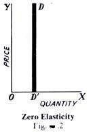
The other extreme limit is when demand is perfectly inelastic. It means that howsoever great the rise or fall in the price of the commodity in question, its demand remains absolutely unchanged. In Fig. 2, the vertical line DD’ shows a perfectly inelastic demand. In other words, in this case elasticity of demand is zero. No amount of change in price induces a change in demand.

In the real world, there is no commodity the demand for which may be absolutely inelastic, i.e., changes in its price will fail to bring about any change at all in the demand for it. Some extension/contraction is bound to occur that is why economists say that elasticity of demand is a matter of degree only. In the same manner, there are few commodities in whose case the demand is perfectly elastic. Thus, in real life, the elasticity of demand of most goods and services lies between the two limits given above, viz., infinity and zero. Some have highly elastic demand while others have less elastic demand.

(c) Very Elastic Demand

Demand is said to be very elastic when even a small change in the price of a commodity leads to a considerable extension/con­traction of the amount demanded of it. In Fig. 3, DD’ curve illustrates such a demand. As a result of change of T in the price, the quantity demanded extends/contracts by MM’, which clearly is comparatively a large change in demand.

(d) Less Elastic Demand

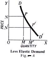
When even a substantial change in price brings only a small extension/contraction in demand, it is said to be less elastic. In Fig. 4, DD’ shows less elastic demand. A fall of NN’ in price extends demand by MM’ only, which is very small.

Significance of Elasticity of Demand:

  • Determination of Output Level

For making production profitable, it is essential that the quantity of goods and services should be produced corresponding to the demand for that product. Since the changes in demand are due to the change in price, the knowledge of elasticity of demand is necessary for determining the output level.

  • Determination of Price

The elasticity of demand for a product is the basis of its price determination. The ratio in which the demand for a product will fall with the rise in its price and vice versa can be known with the knowledge of elasticity of demand.

If the demand for a product is inelastic, the producer can charge high price for it, whereas for an elastic demand product he will charge low price. Thus, the knowledge of elasticity of demand is essential for management in order to earn maximum profit.

  • Price Discrimination by Monopolist

Under monopoly discrimination the problem of pricing the same commodity in two different markets also depends on the elasticity of demand in each market. In the market with elastic demand for his commodity, the discriminating monopolist fixes a low price and in the market with less elastic demand, he charges a high price.

  • Price Determination of Factors of Production

The concept of elasticity for demand is of great importance for determining prices of various factors of production. Factors of production are paid according to their elasticity of demand. In other words, if the demand of a factor is inelastic, its price will be high and if it is elastic, its price will be low.

  • Demand Forecasting

The elasticity of demand is the basis of demand forecasting. The knowledge of income elasticity is essential for demand forecasting of producible goods in future. Long- term production planning and management depend more on the income elasticity because management can know the effect of changing income levels on the demand for his product.

  • Dumping

A firm enters foreign markets for dumping his product on the basis of elasticity of demand to face foreign competition.

  • Determination of Prices of Joint Products

The concept of the elasticity of demand is of much use in the pricing of joint products, like wool and mutton, wheat and straw, cotton and cotton seeds, etc. In such cases, separate cost of production of each product is not known.

Therefore, the price of each is fixed on the basis of its elasticity of demand. That is why products like wool, wheat and cotton having an inelastic demand are priced very high as compared to their byproducts like mutton, straw and cotton seeds which have an elastic demand.

  • Determination of Government Policies

The knowledge of elasticity of demand is also helpful for the government in determining its policies. Before imposing statutory price control on a product, the government must consider the elasticity of demand for that product.

The government decision to declare public utilities those industries whose products have inelastic demand and are in danger of being controlled by monopolist interests depends upon the elasticity of demand for their products.

  • Helpful in Adopting the Policy of Protection

The government considers the elasticity of demand of the products of those industries which apply for the grant of a subsidy or protection. Subsidy or protection is given to only those industries whose products have an elastic demand. As a consequence, they are unable to face foreign competition unless their prices are lowered through sub­sidy or by raising the prices of imported goods by imposing heavy duties on them.

  • Determination of Gains from International Trade

The gains from international trade depend, among others, on the elasticity of demand. A country will gain from international trade if it exports goods with less elasticity of demand and import those goods for which its demand is elastic.

In the first case, it will be in a position to charge a high price for its products and in the latter case it will be paying less for the goods obtained from the other country. Thus, it gains both ways and shall be able to increase the volume of its exports and imports.

Price Elasticity of Demand (PED):

Price Elasticity of Demand measures how much the quantity demanded of a product changes in response to a change in its price. It is calculated using the formula:

PED=% change in quantity demanded% change in price\text{PED} = \frac{\%\text{ change in quantity demanded}}{\%\text{ change in price}}

If PED > 1, demand is elastic (responsive to price changes). If PED < 1, demand is inelastic (not responsive). If PED = 1, demand is unitary elastic. For example, if the price of a luxury car drops and sales rise significantly, the demand is elastic. However, for necessities like salt or milk, even a big price rise may not reduce demand much, indicating inelastic demand.

Understanding PED helps businesses set pricing strategies. If demand is inelastic, firms can raise prices to increase total revenue. If it’s elastic, they may lower prices to attract more buyers and increase sales volume. Government agencies also consider PED when imposing taxes.

Income Elasticity of Demand (YED):

Income Elasticity of Demand measures how sensitive the quantity demanded of a good is to a change in consumers’ income. The formula is:

YED=% change in quantity demanded% change in income\text{YED} = \frac{\%\text{ change in quantity demanded}}{\%\text{ change in income}}

If YED > 1, the product is a luxury good, and demand increases more than proportionally with income. If 0 < YED < 1, it’s a normal good, and demand rises with income but at a slower rate. If YED < 0, it is an inferior good, and demand falls as income rises.

For example, as income increases, people may shift from public transport (inferior good) to personal vehicles (normal or luxury goods). Firms use YED to predict sales trends during economic growth or recession. High-income elasticity indicates sales will rise rapidly in prosperous times, while a low or negative elasticity means demand could fall during downturns.

Cross Elasticity of Demand (XED):

Cross Elasticity of Demand measures how the quantity demanded of one good responds to a price change of another related good. It is used to understand the relationship between substitute and complementary goods. The formula is:

XED=% change in quantity demanded of Good A% change in price of Good B\text{XED} = \frac{\%\text{ change in quantity demanded of Good A}}{\%\text{ change in price of Good B}}

If XED > 0, the goods are substitutes (e.g., tea and coffee); a price rise in one increases demand for the other. If XED < 0, the goods are complements (e.g., printers and ink cartridges); a price rise in one reduces demand for the other. If XED = 0, the goods are unrelated.

Businesses analyze XED to predict how a competitor’s price change can impact their own sales. For example, a soft drink company may monitor price changes of rival products to anticipate changes in their own demand. It’s also valuable in pricing bundled products or forming strategic alliances with producers of complementary goods.

Demand Forecasting: Meaning, Need, Objectives and Methods

Demand forecasting is the process of estimating the future demand for a product or service over a specific period. It is a critical component of business planning that helps organizations make informed decisions regarding production, inventory management, pricing, marketing, and resource allocation. Accurate demand forecasting enables businesses to anticipate customer needs, avoid overproduction or underproduction, and optimize operational efficiency.

The goal of demand forecasting is to reduce uncertainty and support strategic planning by predicting how much of a product consumers will be willing and able to purchase in the future. Forecasts are based on a combination of historical sales data, market trends, seasonal patterns, consumer behaviour, and external economic indicators. Businesses may use qualitative methods (like expert opinion and market research) or quantitative methods (like time series analysis, regression models, and machine learning algorithms) depending on the context and available data.

There are different types of demand forecasting, such as short-term forecasting (used for inventory and scheduling), medium-term forecasting (for sales and budget planning), and long-term forecasting (for capacity and expansion decisions). Each serves a specific business purpose.

Effective demand forecasting provides several benefits. It helps reduce costs, improves customer satisfaction through better availability of products, and enhances financial planning by aligning supply with anticipated demand. It also minimizes the risks of stockouts or surplus inventory.

In today’s competitive and dynamic market environment, demand forecasting is essential for gaining a competitive edge, ensuring customer satisfaction, and achieving overall business success. It supports data-driven decision-making and enables organizations to respond proactively to market changes.

Need of Demand Forecasting:

Demand plays a crucial role in the management of every business. It helps an organization to reduce risks involved in business activities and make important business decisions. Apart from this, demand forecasting provides an insight into the organization’s capital investment and expansion decisions.

  • Business Planning and Strategy

Demand forecasting is essential for long-term business planning and the formulation of strategies. It helps managers estimate future demand and align their production, investment, and marketing efforts accordingly. Forecasting provides insights into market trends, consumer behavior, and potential changes in demand patterns. This enables firms to develop strategies that minimize risks and capitalize on growth opportunities. Accurate forecasts guide business decisions regarding expansion, diversification, and resource allocation, thereby supporting sustainable growth and competitive advantage in dynamic business environments.

  • Production Planning and Scheduling

Forecasting demand enables businesses to plan production activities efficiently. It helps determine the quantity of raw materials, machinery, and labor required to meet expected demand. Proper production planning ensures timely delivery of goods, minimizes lead times, and avoids production bottlenecks. It also helps in reducing production costs by optimizing resource utilization. With accurate demand projections, companies can avoid overproduction, which leads to excess inventory, or underproduction, which causes stockouts and customer dissatisfaction. Thus, forecasting is crucial for streamlined operations.

  • Financial Planning and Budgeting

Demand forecasting plays a critical role in financial planning. It helps businesses estimate future revenues and costs, which is vital for preparing budgets, managing cash flows, and assessing profitability. Accurate forecasts allow firms to anticipate financial needs, allocate funds appropriately, and plan for future investments. It also aids in obtaining credit and financial support, as lenders often require evidence of projected demand and income. In essence, demand forecasting supports better fiscal discipline and long-term financial health of an organization.

  • Inventory Management

Proper demand forecasting ensures effective inventory management. By predicting the demand accurately, businesses can maintain optimum stock levels — not too high to incur carrying costs, and not too low to miss sales opportunities. It prevents situations of excess inventory that can lead to wastage, especially for perishable goods, and also avoids stockouts that frustrate customers. Forecasting aligns inventory control with market demand, thus ensuring product availability while keeping storage costs and capital investment in inventory at manageable levels.

  • Human Resource Planning

Accurate demand forecasts help determine labor requirements for upcoming production and sales activities. Businesses can estimate the number and types of employees needed during peak and off-peak seasons. For example, retailers hire more staff during festive seasons based on expected demand. This ensures optimal workforce allocation, better scheduling, and reduced employee downtime. Demand forecasting thus supports human resource planning by aligning labor supply with demand, ensuring that operations are smooth, cost-effective, and responsive to customer needs.

  • Marketing and Promotional Strategy

Forecasting demand is crucial for developing effective marketing campaigns and promotional activities. By knowing when and where demand is likely to rise, companies can focus their marketing efforts strategically. It enables them to allocate budgets, select appropriate channels, and time promotions to boost sales. For example, a forecasted surge in demand during holidays helps firms plan discounts or advertising campaigns in advance. In this way, demand forecasting improves marketing ROI and strengthens customer engagement and brand positioning.

  • Pricing Decisions

Demand forecasting provides critical input for pricing decisions. Understanding demand elasticity helps firms decide whether to raise or lower prices to maximize revenue. If forecasts show high future demand, businesses may maintain or increase prices. In contrast, if demand is expected to fall, they may consider promotional pricing or discounts. Accurate forecasting allows for dynamic pricing strategies that align with market conditions and consumer expectations, helping businesses stay competitive while optimizing profit margins.

  • Risk Management and Crisis Preparation

One of the most important needs of demand forecasting is to manage business risks. Forecasts allow firms to anticipate shifts in demand due to economic changes, competitor actions, or consumer preferences. This preparation helps companies develop contingency plans, adjust operations, and adapt their offerings accordingly. For instance, during uncertain periods like pandemics or economic slowdowns, forecasting enables proactive decision-making. It enhances organizational resilience by reducing uncertainty and enabling firms to react swiftly to market disruptions.

Objectives of short term demand forecasting:

  • Inventory Management

Short-term demand forecasting helps businesses maintain optimal inventory levels. By predicting near-future demand, firms avoid understocking or overstocking, which reduces storage costs and prevents stockouts. It ensures that inventory is aligned with expected sales, thereby improving customer satisfaction and operational efficiency. Effective inventory planning also minimizes losses due to obsolescence or spoilage, especially for perishable or seasonal products.

  • Production Planning

Short-term forecasts are crucial for daily or weekly production scheduling. They allow businesses to adjust their production volume based on immediate market demand. This prevents overproduction, reduces idle time, and ensures efficient use of resources. Production planning based on accurate short-term forecasts also helps maintain quality control and timely delivery, which are essential for meeting customer expectations and reducing operational costs.

  • Labor Force Scheduling

Forecasting short-term demand allows businesses to align their workforce requirements with production and service needs. Companies can schedule shifts, plan overtime, or hire temporary workers during peak periods. It ensures optimal manpower utilization and prevents labor shortages or surpluses. This leads to cost-effective operations and maintains employee satisfaction by avoiding overburdening during high-demand periods or underemployment during low-demand phases.

  • Pricing Adjustments

Short-term demand forecasting helps in making timely pricing decisions. If a surge in demand is anticipated, businesses may increase prices to maximize profits. Conversely, during a slowdown, they might offer discounts or promotions to stimulate demand. This flexibility in pricing ensures competitiveness, helps clear inventory, and supports revenue targets. Effective pricing adjustments based on demand help maintain a stable market position.

  • Marketing Campaigns

Forecasting demand over the short term helps businesses time their marketing and promotional activities for maximum impact. If demand is expected to rise, promotional efforts can be intensified to boost brand visibility. During slow periods, targeted campaigns can help stimulate customer interest. Proper timing of promotions improves return on marketing investment and ensures better alignment between marketing strategy and consumer behavior.

  • Financial Planning

Short-term forecasting supports accurate cash flow and budget planning. By estimating near-future sales and expenses, firms can manage working capital, schedule purchases, and plan for short-term financing needs. It reduces the likelihood of liquidity issues and ensures smooth operations. Financial planning based on short-term forecasts allows for timely payment of obligations, better credit management, and informed decision-making regarding short-term investments.

  • Customer Service Management

Short-term demand forecasting ensures products and services are available when customers need them. This helps improve order fulfillment rates, reduce waiting times, and enhance customer satisfaction. Meeting customer demand promptly builds trust and loyalty. It also enables businesses to handle sudden demand spikes efficiently, ensuring they remain responsive and competitive in fast-moving markets.

  • Managing Seasonal and Promotional Demand

Short-term forecasts are essential for anticipating seasonal variations and promotional event impacts. For example, demand often spikes during festivals or clearance sales. Accurate forecasting allows companies to prepare in advance, stocking up on popular products and aligning logistics accordingly. This minimizes disruption, boosts sales, and ensures timely service delivery during high-demand periods.

Objectives of long term demand forecasting:

  • Strategic Business Planning

Long-term demand forecasting provides the foundation for strategic decision-making. It helps businesses plan future goals, set long-term objectives, and align operations with projected market trends. Accurate forecasts enable companies to anticipate industry changes, customer needs, and competitive pressures, helping them maintain a sustainable competitive advantage. It supports decisions related to diversification, globalization, and product innovation over extended time horizons.

  • Capital Investment Decisions

Businesses rely on long-term demand forecasting to plan for capital investments such as new plants, machinery, technology upgrades, or infrastructure development. These decisions require large financial commitments and long gestation periods. Forecasting helps determine whether anticipated demand justifies such investments. It ensures that resources are not wasted on underutilized assets and enables the organization to plan investments that support future capacity needs.

  • Capacity Planning

To meet future demand effectively, firms need to plan their production and operational capacity well in advance. Long-term forecasting helps determine when and how much to expand capacity. It guides decisions about scaling production lines, adding shifts, or establishing new facilities. This ensures businesses are prepared to meet future demand increases without facing operational bottlenecks or sacrificing customer service quality.

  • Research and Development (R&D) Planning

Long-term forecasts inform decisions regarding research and development. Businesses can identify future market needs and begin working on new products or improving existing ones. This planning ensures that companies are not reactive but proactive, launching innovative solutions at the right time. R&D planning based on demand projections helps businesses remain technologically advanced and responsive to evolving consumer preferences.

  • Human Resource Development

Long-term forecasting supports workforce planning and development strategies. It helps organizations estimate future staffing needs, plan recruitment drives, invest in employee training, and develop succession plans. This ensures that the business has the right talent and skills available when needed. Preparing a future-ready workforce reduces the risk of talent shortages and helps organizations stay competitive and productive in the long run.

  • Financial Forecasting and Capital Allocation

Forecasting long-term demand assists in financial forecasting and efficient capital allocation. It helps determine future revenue streams, investment priorities, and funding requirements. Businesses can prepare long-term budgets, secure financing in advance, and allocate capital to areas with the highest expected returns. Long-term financial stability is strengthened when capital planning aligns with realistic demand estimates.

  • Risk Management and Contingency Planning

Long-term demand forecasting allows businesses to identify potential risks, such as market downturns, raw material shortages, or technological disruptions. Companies can then create contingency plans to mitigate these risks in advance. This proactive approach enhances organizational resilience, supports crisis readiness, and enables smoother operations even in uncertain or volatile environments.

  • Expansion and Diversification Strategy

Businesses aiming to grow through market expansion or diversification use long-term demand forecasting to identify viable opportunities. Forecasts indicate potential markets, emerging customer segments, and product demand trends. These insights support decisions on entering new geographic areas, launching new product lines, or acquiring complementary businesses. Long-term planning ensures resources are directed toward sustainable growth areas.

Methods of Demand Forecasting:

There is no easy or simple formula to forecast the demand. Proper judgment along with the scientific formula is needed to correctly predict the future demand for a product or service. Some methods of demand forecasting are discussed below:

1. Survey of Buyer’s Choice

When the demand needs to be forecasted in the short run, say a year, then the most feasible method is to ask the customers directly that what are they intending to buy in the forthcoming time period. Thus, under this method, the potential customers are directly interviewed. This survey can be done in any of the following ways:

  • Complete Enumeration Method: Under this method, nearly all the potential buyers are asked about their future purchase plans.
  • Sample Survey Method: Under this method, a sample of potential buyers is chosen scientifically and only those chosen are interviewed.
  • End-use Method: It is especially used for forecasting the demand of the inputs. Under this method, the final users i.e. the consuming industries and other sectors are identified. The desirable norms of consumption of the product are fixed, the targeted output levels are estimated and these norms are applied to forecast the future demand of the inputs.

Hence, it can be said that under this method the burden of demand forecasting is on the buyer. However, the judgments of the buyers are not completely reliable and so the seller should take decisions in the light of his judgment also.

The customer may misjudge their demands and may also change their decisions in the future which in turn may mislead the survey. This method is suitable when goods are supplied in bulk to industries but not in the case of household customers.

2. Collective Opinion Method

Under this method, the salesperson of a firm predicts the estimated future sales in their region. The individual estimates are aggregated to calculate the total estimated future sales. These estimates are reviewed in the light of factors like future changes in the selling price, product designs, changes in competition, advertisement campaigns, the purchasing power of the consumers, employment opportunities, population, etc.

The principle underlying this method is that as the salesmen are closest to the consumers they are more likely to understand the changes in their needs and demands. They can also easily find out the reasons behind the change in their tastes.

Therefore, a firm having good sales personnel can utilize their experience to predict the demands. Hence, this method is also known as Salesforce opinion or Grassroots approach method. However, this method depends on the personal opinions of the sales personnel and is not purely scientific.

3. Barometric Method

This method is based on the past demands of the product and tries to project the past into the future. The economic indicators are used to predict the future trends of the business. Based on the future trends, the demand for the product is forecasted. An index of economic indicators is formed. There are three types of economic indicators, viz. leading indicators, lagging indicators, and coincidental indicators.

The leading indicators are those that move up or down ahead of some other series. The lagging indicators are those that follow a change after some time lag. The coincidental indicators are those that move up and down simultaneously with the level of economic activities.

4. Market Experiment Method

Another one of the methods of demand forecasting is the market experiment method. Under this method, the demand is forecasted by conducting market studies and experiments on consumer behavior under actual but controlled, market conditions.

Certain determinants of demand that can be varied are changed and the experiments are done keeping other factors constant. However, this method is very expensive and time-consuming.

5. Expert Opinion Method

Usually, the market experts have explicit knowledge about the factors affecting the demand. Their opinion can help in demand forecasting. The Delphi technique, developed by Olaf Helmer is one such method.

Under this method, experts are given a series of carefully designed questionnaires and are asked to forecast the demand. They are also required to give the suitable reasons. The opinions are shared with the experts to arrive at a conclusion. This is a fast and cheap technique.

6. Statistical Methods

The statistical method is one of the important methods of demand forecasting. Statistical methods are scientific, reliable and free from biases. The major statistical methods used for demand forecasting are:

  • Trend Projection Method: This method is useful where the organization has sufficient amount of accumulated past data of the sales. This date is arranged chronologically to obtain a time series. Thus, the time series depicts the past trend and on the basis of it, the future market trend can be predicted. It is assumed that the past trend will continue in future. Thus, on the basis of the predicted future trend, the demand for a product or service is forecasted.
  • Regression Analysis: This method establishes a relationship between the dependent variable and the independent variables. In our case, the quantity demanded is the dependent variable and income, the price of goods, price of related goods, the price of substitute goods, etc. are independent variables. The regression equation is derived assuming the relationship to be linear. Regression Equation: Y = a + bX. Where Y is the forecasted demand for a product or service.

Benefits of Forecasting:

  • Future oriented

It enables managers to visualize and discount future to the present. It, thus, improves the quality of planning. Planning is done for future under certain known conditions and forecasting helps in knowing these conditions. It provides knowledge of planning premises with which managers can analyse their strengths and weaknesses and take action to meet the requirements of the future market.

For example, if the TV manufacturers feel that LCD or Plasma televisions will replace the traditional televisions, they should take action to either change their product mix or start manufacturing LCD/Plasma screens. Forecasting, thus, helps in utilizing resources in the best and most profitable business areas.

In the fast changing technological world, businesses may find it difficult to survive if they do not forecast customers’ needs and competitors’ moves.

  • Identification of critical areas

Forecasting helps in identifying areas that need managerial attention. It saves the company from incurring losses because of bad planning or ill defined objectives. By identifying critical areas of management and forecasting the requirement of different resources like money, men, material etc., managers can formulate better objectives and policies for the organisation. Forecasting, thus, increases organisational and managerial efficiency in terms of framing and implementing organisational plans and policies.

  • Reduces risk

Though forecasting cannot eliminate risk, it reduces it substantially by estimating the direction in which environmental factors are moving. It helps the organisation survive in the uncertain environment by providing clues about what is going to happen in future.

If managers know in advance about changes in consumer preferences, they will bring required modifications in their product design in order to meet the changed expectations of the consumers. Thus, forecasting cannot stop the future changes from happening but it can prepare the organisations to face them when they occur or avoid them, if they can.

  • Coordination

Forecasting involves participation of organisational members of all departments at all levels. It helps in coordinating departmental plans of the organisation at all levels. People in all departments at all levels are actively involved in coordinating business operations with likely future changes predicted as a result of forecasting. Thus, forecasting helps in movement of all the plans in the same direction.

  • Effective management

By identifying the critical areas of functioning, managers can formulate sound objectives and policies for their organisations. This increases organisational efficiency, effectiveness in achieving the plans, better management and effective goal attainment.

  • Development of executives

Forecasting develops the mental, conceptual and analytical abilities of executives to do things in planned, systematic and scientific manner. This helps to develop management executives.

error: Content is protected !!