Iso-Product Curves- Meaning and Features

An iso-product curve is locus of various combinations of two factors of production giving the same level of output and a producer is indifferent to each of such combinations. All the combinations of two inputs give the same quantum of output to a producer and the producer is indifferent to each such combination. He does not have any preference. These iso-product curves are also called production indifference curves. The concept of iso-product curve can be explained with the help of iso-quant schedule and diagram.

Assumptions:

The main assumptions of Iso-quant curves are as follows:

1. Two Factors of Production:

Only two factors are used to produce a commodity.

2. Divisible Factor:

Factors of production can be divided into small parts.

3. Constant Technique:

Technique of production is constant or is known beforehand.

4. Possibility of Technical Substitution:

The substitution between the two factors is technically possible. That is, production function is of ‘variable proportion’ type rather than fixed proportion.

5. Efficient Combinations:

Under the given technique, factors of production can be used with maximum efficiency.

Iso-Quant Schedule

An iso-quant schedule shows different combinations of two factors of production (inputs) at which a producer gets equal quantum of output.

The schedule is given below:

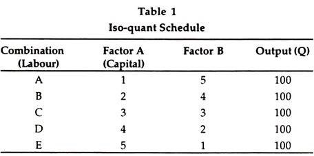
The above schedule shows the different combinations of two inputs, namely, labour and capital and the resultant output 100 units from each combination. The units of labour are increasing and units of capital are decreasing but the quantity of output remains the same.

The schedule can be depicted in the form of a diagram given below:

In the diagram factor A and factor B are shown on OX-axis and OY-axis respectively. IP is the iso-product curve showing the different combinations (A, B, C, D and E) of the two factors of production giving the same quantity of output (100 units).

The IP curve slopes downward to the right. It explains with the increase in the units of factor-A when we are reducing the units of factor-B.

Iso-Product Curve and Indifference Curve

The shape and slope of iso-product curve and indifference curve are similar but both of them have the following differences:

(1) Iso-product curve shows the quantum of output while an indifference curve shows the level of satisfaction. Iso-product curve shows the different combinations of two factors of production (inputs) showing the same quantum of output but an indifference curve shows the different combinations of two commodities showing the same level of satisfaction.

(2) We can prepare an iso-product map by which we can express that how much less or more quantity of output is shown by each iso-product curve but an indifference curve cannot say how much more or less is the satisfaction from different combinations of two commodities a consumer is getting. Utility or satisfaction is not measurable but the quantity of output is measurable with the help of iso-product curve.

Features of Iso-Product Curves

The following are the characteristics of iso-product curves:

(1) Iso-Product Curves Slope Downward to the Right

Iso- product curves slope downward to the right because producer has limited resources with alternative uses and he is faced with the problem of choice. He cannot increase the amount of labour and capital. If he employs more of labour he has to employ less of capital in order to get the same level of output as given in the following diagram:

The diagram shows that units of labour are shown on OX- axis and units of capital on OY-axis. A combination shows OK of capital and OL of labour while at B combination OK₁ of capital and OL₁ of labour showing the same amount of output (100 units). But the producer has employed more of labour and less of capital and on account of it the iso-product curve slopes downward to the right.

(2) Iso-Product Curves are Convex to the Origin

As an indifference curve is convex to the origin, similarly an iso-product curve is also convex to the origin. In an iso-product curve a factor of production is substituted by another factor of production and consequently the marginal rate of technical substitution of labour for capital (MRTS_LK) declines and on account of decreasing MRTS_LK the iso-product curves are convex to the origin.

It is shown by the following diagram:

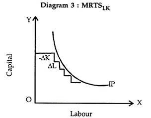
The table reveals that we are increasing the units of labour and reducing the units of capital. The MRTS_LK shows a declining trend.

(3) Two Iso-Product Curve never Intersect Each Other

Another characteristic is that two iso-product curves do not intersect each other as different iso-product curves show different level of output.

It is shown by the following diagram:

Capital and labour are shown on OY-axis and OX-axis respectively. IP and IP_X are two iso-product curves. E is the point where IP₂ and IP₁ intersect each other.

Before E point IP₁ is higher than IP₂ and after E point IP₁ is higher than IP. In such a situation it is difficult to know which Iso- product curve gives higher level of output. Hence, we can say that it is indeterminate and two iso-product curves do not cut each other.

(4) Higher the Iso-Quant Curve Higher is the Level of Output

A producer gets the same level of output with different combinations of two inputs on the iso-product curve. But in case of different iso-product curves the level of output differs. Higher the iso-product curve, higher the level of output and lower the iso-product, lower will be the level of output. It can be seen from Diagram 5.

The diagram shows Iso-product map in which three Iso- product curves are showing different levels of output. IP, IP₁ and IP₂ are showing 500 units, 1000 units and 1500 units respectively which show increasing trends. Higher the iso-product curve higher is the level of output (IP to IP₂), lower the iso-product curve lower will be the level of output (IP₂ to IP). The highest iso-product curve is IP₂ and the lowest iso-product curve is IP.

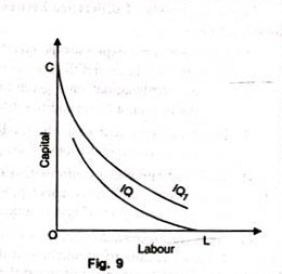
(5) No Isoquant can Touch Either Axis:

If an isoquant touches X-axis, it would mean that the product is being produced with the help of labour alone without using capital at all. These logical absurdities for OL units of labour alone are unable to produce anything. Similarly, OC units of capital alone cannot produce anything without the use of labour. Therefore as seen in figure 9, IQ and IQ1 cannot be isoquants.

(6) Each Isoquant is Oval-Shaped.

It means that at some point it begins to recede from each axis. This shape is a consequence of the fact that if a producer uses more of capital or more of labour or more of both than is necessary, the total product will eventually decline. The firm will produce only in those segments of the isoquants which are convex to the origin and lie between the ridge lines. This is the economic region of production. In Figure 10, oval shaped isoquants are shown.

Curves OA and OB are the ridge lines and in between them only feasible units of capital and labour can be employed to produce 100, 200, 300 and 400 units of the product. For example, OT units of labour and ST units of the capital can produce 100 units of the product, but the same output can be obtained by using the same quantity of labour T and less quantity of capital VT.

Thus only an unwise entrepreneur will produce in the dotted region of the iso-quant 100. The dotted segments of an isoquant are the waste- bearing segments. They form the uneconomic regions of production. In the up dotted portion, more capital and in the lower dotted portion more labour than necessary is employed. Hence GH, JK, LM, and NP segments of the elliptical curves are the isoquants.

Marginal Rate of Technical Substitution (MRTS)

Marginal rate of technical substitution is an important concept in the study of iso-product curve analysis.

The marginal rate of technical substitution is the rate at which two factors of production (inputs) are substituted. For example, we have two factors of production—capital and labour. The marginal rate of technical substitution of labour for capital (MRTS_LK) is that rate at which one unit of labour substitutes the number of units of capital.

The MRTS_LK can be studied from the following table:

The table reveals that all the combinations of factor A (labour) and factor B (capital) give the same level of output. If he has C combination then 1A+12B will give the same level of output when he employs 5 units of A and 2 units of B (5A+2B) at G combination the level of output remains unchanged. Hence, the marginal rate of technical substitution of factor A for factor B can be written mathematically in the following formula:

MRTS_ab = ΔB/ΔA

Thus the MRTS_AB shows the marginal rate of technical substitution of A factor for B factor.

Generally, the MRTS declines because as we employ more of factor A then we have to employ less of factor B. It is called the MRTS and each iso-product is conveyed to origin on account of declining MRTS.

Iso-Cost Curve

Different combinations of two inputs give the same level of output which is shown by an iso-product curve. Higher the iso-product curve higher will be the level of output. A producer is faced with the problem of choice because his resources are limited and they have alternative uses.

The choice of a producer depends upon the resources at his disposal and the factor prices. An iso-cost curve shows the various combinations of two inputs (labour and capital) that can be employed by a producer with his given resources. It means the resources of a producer and price of two inputs are shown by this curve. It is given in the Diagram 6.

The diagram shows labour and capital on OX-axis and OY- axis respectively. AB, A₁B₁ and A₂B₂ are iso-cost line or curves showing different combinations of labour and capital. If the producer wants to employ more of labour and capital then he should keep in his mind his budget and the prices of both these factors. Higher the iso-cost curve higher will be the need for resources. Iso-cost curve is also known as outlay line, input price line and factor cost