Author: indiafreenotes

Firm Demand (company demand) denotes the demand for the product/s of a particular firm. While Industry demand means the demand for the product of a particular industry. An industry comprises all the firms or companies producing similar products which are quite close substitutes to each other irrespective of the differences in their brand names. To understand the relation between company and industry demand necessitates an understanding of different market structures.

1. Demand Curve under Perfect competition

Under Perfect Competition industry demand is completely different from the individual firm demand. The industry demand curve is downward sloping. The price in the market is determined by the interactions of the forces of demand and supply. The point of intersection between demand and supply curves determines the equilibrium price of the product. Now the number of firms under Perfect Competition is so large that a single firm has no influence on either the total output or the price. Its contribution to total output is just microscopic. If a new firm enters or an existing firm takes an exit the total output does not get affected much. A firm under Perfect Competition cannot fix the price of its product. It will have to sell its product at the going market price as it is determined by demand and supply forces in the market. A firm under Perfect Competition is a price taker and not a price maker. Price is given to the firms and each unit of its output is sold at the given market price and thus the demand curve of firm or its average revenue curve becomes horizontal. Horizontality of average revenue curve (demand curve) is the acid test of a firm under Perfect Competition.

Nature of Demand Curve under Perfect competition

In case of perfect competition, there are very large no. of buyers and sellers selling a homogeneous product at a price fixed by the market. Therefore, each firm is a price taker and faces a perfectly elastic demand curve.

2. Demand Curve under Monopolistic competition

Under Monopolistic Competition there is competition among a group of monopolists producing differentiated product. The product of each firm is slightly different from that of other. There are also substitutes and therefore the demand curve of each firm’s product is downward sloping and is relatively elastic in nature. In monopolistic competition there are many sellers with differentiated product and hence industry demand curve hardly has any meaning.

Nature of Demand Curve under Monopolistic competition

Under monopolistic competition, large no. of firms selling closely related but differentiated products makes the demand curve downward sloping. It implies that a firm can sell more output only by reducing the price of its product.

3. Demand Curve under Monopoly competition

The demand curve of an individual firm is not the same as the industry or market demand curve except in case of monopoly. Monopoly is that market category in which there is only a single seller and therefore there is no difference between a firm and an industry. The firm is itself an industry and therefore the demand curve of the individual firm as well as the industry demand curve under monopoly will be the same and as we shall see later is downward sloping. Moreover as there are no close substitutes under monopoly the demand curve is relatively steeper showing relatively inelastic demand under monopoly.

Nature of Demand Curve under Monopoly competition

A monopoly firm is like an industry as the single seller constitutes the entire market for the product, which has no close substitutes. So, a monopolist has full freedom and power to fix price for the product. However, demand of the product is not in the control of monopoly firm. In order to increase the output to be sold, the monopolist will have to reduce the price. Therefore, monopoly firm faces a downward sloping demand curve.

4. Demand Curve under oligopoly competition

In case of Oligopoly market there are few sellers producing either differentiated or homogenous products. The demand for a firm’s product is influenced by the actions of its rivals. The demand curve of a firm under oligopoly has a kink.

Nature of Demand Curve under oligopoly competition

The demand curve for an oligopoly firm is indeterminate, i.e. it cannot be drawn accurately as exact behavior pattern of a producer cannot be ascertained with certainty.

It’s human nature. If the price of a product goes up, consumers buy less of it. If the price goes down, consumers buy more. In economic terms, that’s called price elasticity. But what if the price of gasoline goes up, the gas tank in your SUV is on empty, and you have to be at work in 20 minutes? Will you refuse to buy gasoline because the price is high? Of course not. You don’t have any alternative, so you pay the higher price, buy the needed quantity of gasoline and go to your job. That’s called price inelasticity.

Price Elasticity

Price elasticity measures the changes in demand for a product in reaction to changes in the price for that product. It’s a ratio of percentages, and the formula is as follows:

Price elasticity of demand = Percentage change in demand ÷ Percentage change in price

When this ratio is greater than one, the price is considered to be elastic, and demand declines as the price increases. When the ratio is less than one, the demand for a product does not change substantially with changes in price. In this case, a company could increase its prices and not suffer a significant decline in sales volume.

Example of Price Elasticity

Let’s suppose that a 10-count box of Quaker Instant Oatmeal sells for $2.18. When the price goes up to $2.59, the demand drops from 500 boxes per week to 350 boxes per week. The elasticity is calculated as follows:

Price elasticity = ((500 – 350)/500) ÷ (($2.18-$2.59)/$2.18)

= (150/500) ÷ ($0.41/$2.18)

= 30 percent ÷ 19 percent

= 1.6

Since the result, 1.6, is greater than one, the price elasticity for an increase in the price of Quaker Oatmeal is high. The price for oatmeal goes up, and consumers buy less of the product. They may start buying other cereal products, or they might switch to the grocery store’s generic brand of oatmeal.

Factors That Affect Elasticity

The factors that affect the price elasticity of any product include:

(i) Substitutes

As in the case of rising prices for oatmeal, consumers can shift their purchases to similar products if they are readily available. Coca-Cola and Pepsi are products that can be easily substituted for each other when prices change. This is an example of elastic demand. If the alternatives are limited, the demand is less elastic.

(ii) Necessities versus luxuries

Necessities are products that people must have regardless of the price. Everyone has to drink water, so if the water company raises prices, people continue to consume and pay for it. Luxuries are optional; they aren’t necessary to live. Large-screen HDTVs are nice to have, but if the prices go up, consumers can put off buying them.

(iii) Share of the consumer’s income

Products that consume a high proportion of a family’s income are sensitive to price increases. A car is a good example. Increases in car prices can cause a family to delay purchasing a new car. They keep their old car longer and make the necessary repairs. However, if a grocery store increases the price of toothpicks, consumers still buy them because the price isn’t a big piece of their income.

(iv) Short-term versus long-term timing

Gasoline is an excellent example of a product that prices inelastic in the short term but elastic in the long term. When gas prices go up, the consumer still has to buy gas to get to work. However, if gas prices stay high for the long term, consumers make changes. They may buy more fuel-efficient cars, set up a carpool with other workers, or start taking a train or bus to work.

Why Elasticity Is Important?

Marketers must have some knowledge about the elasticity of their products to set pricing strategies. If marketers know that the demand for their products is inelastic, then they can raise prices without fear of losing sales. On the other hand, if demand for their products is highly elastic, then raising prices could be a dangerous game.

The relationship between price elasticity and total revenue is an important metric for marketers to understand. Understanding whether the price of a product is elastic or inelastic is essential for a company to develop an effective marketing campaign and survive in the marketplace. Price elasticity is a tool that marketers can use against their competitors to increase their share of a market.

It’s difficult to plan your future sales and success if you don’t have any idea what the appetite is in the marketplace for your goods and services. Although there is no perfect way of predicting what your customers may want to buy in the future, there are some demand estimation methods that can give you a quantifiable idea of what you can expect. While these demand estimation methods vary slightly in how they are implemented, they will help you plan your marketing strategies to account for anticipated sales. Using demand estimation methods, you can gauge how many goods to produce and how many services to offer, and you can also determine whether or not expansion is feasible.

Elements of Demand Estimation

Demand estimation in managerial economics refers to predicting how consumers will behave in relation to your products and services in the future. The estimation is often based on a number of different variables that can include changes in price, changes in how your competition increases or decreases its prices, and economic factors such as a recession, which would affect consumer buying. By applying these variables, you can analyze how your customer’s demands might change for the better or for the worse depending on a specific factor. As a result, you may decide that you can raise prices because demand will remain steady or even increase, or you may decide that you will have to pull back on production because circumstances are not likely to be favorable. Demand estimation in managerial economics is an important way for you to determine the short-term and long-term course of your business.

Methods of Demand Estimation

There are several methods of demand estimation in managerial economics that can help you obtain a clear picture of what might happen to customer demand level in the future. One of the popular steps in demand estimation is to conduct a survey, which often includes focus groups and direct interviews with customers. Surveys are useful because you are obtaining information from your target market and they can tell you their fears, hopes, and future plans. However, there are some drawbacks with this method because customers may tell you what they will do in the future and circumstances could quickly change those purchasing plans. It’s also difficult to get a truly representative sample when you conduct surveys.

Another of the common steps in demand estimation is regression analysis in which a dependent variable such as demand for a product or service is compared to an independent variable such as price. Regression analysis relies heavily on statistics to create a comprehensive picture of future consumer demand based on specific independent variables. A basic regression analysis model will only make comparisons between the dependent variable and one independent variable. A more complex regression analysis model will make comparisons between the dependent variable and multiple independent variables.

Demand Estimation Considerations

Regardless of the steps in demand estimation that you use, it’s important to understand that this process can help you when it comes to pricing and production. When you offer a new product or start a new business, you may not have any idea how to price your product. When you have an idea what the demand will be for the product or service, you know approximately how much you can charge for that product or service. This can help you avoid overpricing your product or service. Demand estimation can also help you with production. For example, if the demand in your market is projected to be for 50,000 units, you can produce enough goods to account for that demand without over-producing. Remember also that these estimations are only educated guesses as to what the demand for a product or service will be. Always allow some room for error in the estimation of the demand for your business or you may be in for some surprises.

Good business decisions are almost always based on fact. Factual data provides a measure of objectivity, even when a decision ultimately comes down to your best educated guess. Although demand estimation is really an educated guess, it can include the use of fact, up to and including a set of complex statistical calculations that can be difficult to understand and to complete. While other available methods may be less scientific, they are also easier to use. Because demand estimation provides crucial information, every business owner should be familiar with the concept and know how to apply estimation results.

The Basics

Demand estimation is a prediction focusing on future consumer behavior. It predicts demand for a business’s products or services by applying a set of variables that show how, for example, price changes, a competitor’s pricing strategy or changes in consumer income levels will affect product demand. Once armed with this information, management can then begin to make strategic business decisions ranging from reviewing pricing strategies to setting product inventory levels to deciding whether to make fixed asset investments and whether to introduce a new product or enter a new market.

1. Survey Method

Consumer interviews, surveys and focus group meetings are a grass-roots method of estimating demand. The method operates under the idea that consumers know themselves best and that interacting with consumers directly is the best way to estimate future product demand. Getting information directly from consumers, however, decreases objectivity and increases the chance of errors. It can be difficult, for example, to get a truly random sample of the target consumer population. Consumer responses may also be biased in that responses may not reflect what a consumer will do, but rather what they would like to do, or a consumer may be unable to provide a precise or accurate response.

2. Market Study Method

Market studies are a direct demand estimation method that combines consumer interaction with science. The process starts by setting a constant, such as price, and variables such as size and/or color. Market studies then display products at, for example, the same price, but in a variety of sizes and locations or settings over a period of time. Once the study is complete, analyzing the results reveals how demand for the product at that price changes according to, in this case, size or color.

3. Regression Analysis Method

Demand estimation can also rely on regression analysis, a statistical way to find the best relationship between a dependent variable in this case, product demand and one or more independent variables, such as price or location. Although fully understanding demand estimation calculations requires a background in statistics, the process is not difficult to understand. Setup starts by identifying and obtaining data, such as cross-sectional market data or results of a time study or consumer survey on the independent variable or variables to be used in the calculation. Next comes choosing between using a simple or multiple regression model, depending on whether the calculation includes one or multiple variables. Both models display demand as an unknown. Parameters such as a specific price or average annual income are set. Statistical calculations can then begin, and management can move on to interpreting results.

It is essential to know the meaning of firm and industry before analyzing the two. Firm is an organization which produces and supplies goods that are demanded by the people with the goal of maximizing its profits.

According to R.L.Miller, “Firm is an organization that buys and hires resources and sells goods and services.” To Lipsey, “Firm is the unit that employs factors of production to produce commodities that it sells to other firms, to households, or to the government.”

Industry is a group of firms producing homogeneous products in a market. According to Lipsey, “Industry is a group of firms that sells a well-defined product or closely related set of products.” For example, Raymond, Maffatlal, Arvind, etc., are cloth manufacturing firms, whereas a group of such firms is called the textile industry.

Conditions of Equilibrium of the Firm and Industry

A firm is in equilibrium when it has no tendency to change its level of output. It needs neither expansion nor contraction. It wants to earn maximum profits in by equating its marginal cost with its marginal revenue, i.e. MC = MR.

Diagrammatically, the conditions of equilibrium of the firm are:

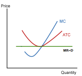
(1) The MC curve must equal the MR curve. This is the first order and necessary condition. But this is not a sufficient condition which may be fulfilled yet the firm may not be in equilibrium.

(2) The MC curve must cut the MR curve from below and after the point of equilibrium it must be above the MR. This is the second order condition.’ Under conditions of perfect competition, the MR curve of a firm coincides with the AR curve. The MR curve is horizontal to the X- axis. Therefore, the firm is in equilibrium when MC=MR=AR (Price).

In Figure 1(A), the MC curve cuts the MR curve first at point A. It satisfies the condition of MC = MR, but it is not a point of maximum profits because after point A, the MC curve is below the MR curve. It does not pay the firm to produce the minimum output OM when it can earn larger profits by producing beyond OM.

Point В is of maximum profits where both the conditions are satisfied. Between points A and B. it pays the firm to expand its output because it’s MR > MC. It will, however, stop further production when it reaches the OM₁ level of output where the firm satisfies both the conditions of equilibrium.

If it has any plans to produce more than OM₁ it will be incurring losses, for its marginal cost exceeds its marginal revenue beyond the equilibrium point B. The same conclusions hold good in the case of a straight line MC curve as shown in Figure 1. (B)

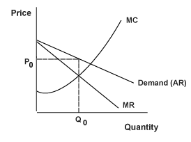
An industry is in equilibrium: firstly when there is no tendency for the firms either to leave or enter the industry, and secondly, when each firm is also in equilibrium. The first condition implies that the average cost curves coincide with the average revenue curves of all the firms in the industry. They are earning only normal profits, which are supposed to be included in the average cost curves of the firms.

The second condition implies the equality of MC and MR. Under a perfectly competitive industry these two conditions must be satisfied at the point of equilibrium, i.e.

MC = MR … (1)

AC = AR … (2)

AR = MR

MC = AC = AR

Such a situation represents full equilibrium of the industry.

Short-Run Equilibrium of the Firm and Industry

SHORT-RUN EQUILIBRIUM OF THE FIRM

A firm is in equilibrium in the short-run when it has no tendency to expand or contract its output and wants to earn maximum profit or to incur minimum losses. The short-run is a period of time in which the firm can vary its output by changing the variable factors of production. The number of firms in the industry is fixed because neither the existing firms can leave nor new firms can enter it.

Assumptions:

This analysis is based on the following assumptions

• All firms use homogeneous factors of production.
• Firms are of different efficiency.
• Cost curves of firms vary from each other.
• All firms sell their products at the same price determined by demand and supply of the industry so that the price of each firm, P (Price) = AR = MR.
• Firms produce and sell different quantities.

The short-run equilibrium of the firm can be explained with the help of marginal analysis and total cost- total revenue analysis.

1. Marginal Cost-Marginal Revenue Analysis

During the short run, a firm will produce only if its price equals the average variable cost or is higher than the average variable cost (AVC). Further, if the price is more than the averages total costs (SAC or АТС), i.e., P— AR > SAC, the firm will be earning supernormal (or abnormal) profits.

If price equals the average total costs, i.e., P = AR = SAC, the firm will be earning normal (or zero) profits or breaks-even. If price equals AVC, the firm will be incurring a loss. If price falls even a little below AVC, the firm will shut down because in order to produce it must cover at least its AVC during the short-run.

So during the short-run under perfect competition, a firm is in equilibrium in all the above noted situations. We illustrate them diagrammatically as under.

(a) Supernormal Profits

The firm will be earning supernormal profits in the short-run when price is higher than the short-run average cost, as shown in Figure 2 (A). The firm is in equilibrium at point E₁ where SMC=MR and SMC cuts MR from below. OQ, is the equilibrium output and OP (=Q₁E₁) is the equilibrium price. Q₁S are the short-run average costs.

SE₁ (=Q₁E₁-Q₁S) is the profit per unit. TS (equilibrium output) (per unit profit) = TSE₁P area is the supernormal profits.

(b) Normal Profits

The firm may earn normal profits when price equals the short-run average costs as shown in Figure 2 (B). The firm is in equilibrium at point E₂ where SMC =MR and SMC cuts MR from below. OQ₂ is the equilibrium output and OP (=Q₂E) is the equilibrium price. The firm is earning normal profits because Price = AR = MR =SMC= SAC at its minimum point E₂.

(c) Minimum Loss

The firm may be in equilibrium and yet incur a loss when price is less than the short-run average costs, as shown in Figure 2 (C). The firm is in equilibrium at point E₃ where SMC = MR and SMC cuts MR from below. OQ₃ is the equilibrium output and OP (=Q₃E₃) is the equilibrium price.

Since the average costs Q₃B are higher than the price Q₃E₃, E₃B is the loss per unit (Q₃B-Q₃E₃). The total loss is PE₃ x E₃B = PE₃BA. The firm will continue to produce OQ₃ output so long as it is covering its average variable cost plus some of its fixed cost.

(d) Maximum Loss

If the price fig. 2 falls to the level of AVC, the firm will just cover its average variable cost, as shown in figure 2 (D). It is indifferent whether to operate or close down because its losses are the maximum.

It will pay such a firm to continue producing OQ₄ output and incur PE₄GF losses rather than close down in the short-run. OQ₄ is the shutdown output because if the price falls below OP, the firm will stop production. E₄ is, therefore, the shutdown point.

(e) Shut Down Stage

Figure 2. (E) shows a firm which is unable to cover even its AVC at OQ₀ level of output because the price OP is below the AVC curve. It must shut down.

Thus in the short-run, there are firms which earn normal profits, supernormal profits and incur losses.

2. Total Cost-Total Revenue Analysis

The short-run equilibrium of the firm can also he shown with the help of total cost and total revenue curves. The firm is able to maximize its profits when the positive difference between TR and TC is the greatest. This is shown in Figure 3 where TR is the total revenue curve and TC the total cost curve.

The total revenue curve is an upward sloping straight line curve starting from O. This is because the firm sells small or large quantities of its product at a constant price under perfect competition. If the firm produces nothing, total revenue will be zero the more it produces, the larger is the increase in total revenue. Hence the TR curve is linear and slopes upward.

The firm will maximize its profits at that level of output where the gap between the TR curve and the TC curve is the maximum. Geometrically, it is that level at which the slope of a tangent drawn to the total cost curve equals the slope of the total revenue curve. In Figure 3, the maximum amount of profit is measured by TP at OQ output.

At outputs smaller or larger than OQ between A and B points, the firm’s profits shrink. If the firm produces OQ₁ output, its losses are the maximum because the TC curve is above the TR curve. At Q₁ its profits are zero.

This is the break-even point of the firm. It starts earning profits when it produces beyond OQ₁ output level. At OQ₂ level, its profits are again zero. If it produces beyond this level, it incurs losses because TC > TR.

SHORT-RUN EQUILIBRIUM OF THE INDUSTRY

An industry is in equilibrium in the short-run when its total output remains steady, there being no tendency to expand or contract its output. If all firms are in equilibrium, the industry is also in equilibrium. For full equilibrium of the industry in the short-run, all firms must be earning only normal profits.

The condition for this is SMC = MR = AR = SAC. But full equilibrium of the industry is by sheer accident because in the short- run some firms may he earning supernormal profits and some incurring losses. Even then, the industry is in short-run equilibrium when its quantity demanded and quantities supplied are equal at the price which clears the market.

This is illustrated in Figure 4 where in Panel (A), the industry is in equilibrium at point E where its demand curve D and supply curve S intersect which determine OP price at which its total output OQ is cleared. But at the prevailing price OP, some firms are earning supernormal profits PE₁ST, as shown in Panel (B), while some other firms are incurring FGE₂P losses, as shown in Panel (C) of the figure.

Long-Run Equilibrium of the Firm and Industry

LONG-RUN EQUILIBRIUM OF THE FIRM

The long run is a period of time in which the firm can change its plant and scale of operations. Thus in the long-run all costs are variable and there are no fixed costs. The firm is in the long-run equilibrium under perfect competition when it does not want to change its equilibrium output.

It is earning normal profits. If some firms are earning supernormal profits, new firms will enter the industry and supernormal profits will be competed away. If some firms are incurring losses, some of the firms will leave the industry till all earn normal profits.

Thus there is no tendency for firms to enter or leave the industry because every firm must earn normal profits. “In the long-run, firms are in equilibrium when they have adjusted their plant so as to produce at the minimum point of their long-run AC curve, which is tangent (at this point) to the demand (AR) curve defined by the market price” so that they earn normal profits.

Assumptions

This analysis is based on the following assumptions

• Firms are free to enter into or leave the industry.
• All firms are of equal efficiency.
• All factors are homogenous. They can be obtained at constant and uniform prices. SMC
• Cost curves of firms are uniform.
• The plants of firms are equal, having given technology.
• All firms have perfect knowledge about price and output.

Given these assumptions, each firm of the industry will be in long-run equilibrium when it fulfils the following two conditions.

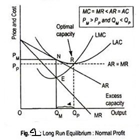
(1) In equilibrium, its short-run marginal cost (SMC) must equal to its long-run marginal cost (LMC) as well as its short-run average cost (SAC) and its long-run average cost (LAC) and both should equal MR=AR=P.

Thus the first equilibrium condition is

SMC = LMC = MR = AR = P = SAC = LAC at its minimum point, and

(2) LMC curve must cut MR curve from below: Both these conditions of equilibrium are satisfied at point E in Figure 5 where SMC and LMC curves cut from below SAC and LAC curves at their minimum point E and SMC and LMC curves cut AR = MR curve from below. All curves meet at this point E and the firm produces OQ optimum output and sells it at OP price.

Since we assume equal costs of all the firms of industry, all firms will be in equilibrium in the long-run. At OP price a firm will have neither a tendency to neither leave nor enter the industry and all firms will earn normal profits.

LONG-RUN EQUILIBRIUM OF THE INDUSTRY

The industry is in equilibrium in the long-run when all firms earn normal profits. There is no incentive for firms to leave the industry or for new firms to enter it. With all factors homogeneous and given their prices and the same technology, each firm and industry as a whole are in full equilibrium where LMC = MR = AR (-P) = LAC at its minimum.

Such an equilibrium position is attained when the long-run price for the industry is determined by the equality of total de­mand and supply of the industry.

The long-run equi­librium of the industry is illustrated in Figure 6 (A) where the long-run price OP is determined by the intersection of the demand curve D and the supply curve S at point E and the industry is producing OM output. At this price OP, the firms are in equilibrium at point A in Panel (B) at OQ level of output where LMC = SMC = MR =P ( = AR) = SAC = LAC at its minimum.

At this level, the firms are earning normal profits and have no incentive to enter or leave the industry. It follows that when the industry is in long-run equilibrium, each firm in the industry is also in long-run equilibrium. If both the industry and the firms are in long-run equilibrium, they are also in short-run equilibrium.

A monopoly refers to when a company and its product offerings dominate one sector or industry. Monopolies can be considered an extreme result of free-market capitalism in that absent any restriction or restraints, a single company or group becomes large enough to own all or nearly all of the market (goods, supplies, commodities, infrastructure, and assets) for a particular type of product or service. The term monopoly is often used to describe an entity that has total or near-total control of a market.

Monopolies typically have an unfair advantage over their competition since they are either the only provider of a product or control most of the market share or customers for their product. Although monopolies might differ from industry-to-industry, they tend to share similar characteristics that include:

• High or no barriers to entry: Competitors are not able to enter the market, and the monopoly can easily prevent competition from developing their foothold in an industry by acquiring the competition.
• Single seller: There is only one seller in the market, meaning the company becomes the same as the industry it serves.
• Price maker: The company that operates the monopoly decides the price of the product that it will sell without any competition keeping their prices in check. As a result, monopolies can raise prices at will.
• Economies of scale: A monopoly often can produce at a lower cost than smaller companies. Monopolies can buy huge quantities of inventory, for example, usually a volume discount. As a result, a monopoly can lower its prices so much that smaller competitors can’t survive. Essentially, monopolies can engage in price wars due to their scale of their manufacturing and distribution networks such as warehousing and shipping, that can be done at lower costs than any of the competitors in the industry.

Monopolistic competition characterizes an industry in which many firms offer products or services that are similar, but not perfect substitutes. Barriers to entry and exit in a monopolistic competitive industry are low, and the decisions of any one firm do not directly affect those of its competitors. Monopolistic competition is closely related to the business strategy of brand differentiation.

Monopolistic competition is a middle ground between monopoly and perfect competition (a purely theoretical state), and combines elements of each. All firms in monopolistic competition have the same, relatively low degree of market power; they are all price makers. In the long run, demand is highly elastic, meaning that it is sensitive to price changes. In the short run, economic profit is positive, but it approaches zero in the long run. Firms in monopolistic competition tend to advertise heavily.

Monopolistic competition is a form of competition that characterizes a number of industries that are familiar to consumers in their day-to-day lives. Examples include restaurants, hair salons, clothing, and consumer electronics.

Features of monopolistic competition

The main features of monopolistic competition are as under:

1. Large Number of Buyers and Sellers

There are large number of firms but not as large as under perfect competition.

That means each firm can control its price-output policy to some extent. It is assumed that any price-output policy of a firm will not get reaction from other firms that means each firm follows the independent price policy.

If a firm reduces its price, the gains in sales will be slightly spread over many of its rivals so that the extent to which each of the rival firms suffers will be very small. Thus these rival firms will have no reason to react.

2. Free Entry and Exit of Firms

Like perfect competition, under monopolistic competition also, the firms can enter or exit freely. The firms will enter when the existing firms are making super-normal profits. With the entry of new firms, the supply would increase which would reduce the price and hence the existing firms will be left only with normal profits. Similarly, if the existing firms are sustaining losses, some of the marginal firms will exit. It will reduce the supply due to which price would rise and the existing firms will be left only with normal profit.

3. Product Differentiation

Another feature of the monopolistic competition is the product differentiation. Product differentiation refers to a situation when the buyers of the product differentiate the product with other. Basically, the products of different firms are not altogether different; they are slightly different from others. Although each firm producing differentiated product has the monopoly of its own product, yet he has to face the competition. This product differentiation may be real or imaginary. Real differences are like design, material used, skill etc. whereas imaginary differences are through advertising, trade mark and so on.

4. Selling Cost

Another feature of the monopolistic competition is that every firm tries to promote its product by different types of expenditures. Advertisement is the most important constituent of the selling cost which affects demand as well as cost of the product. The main purpose of the monopolist is to earn maximum profits; therefore, he adjusts this type of expenditure accordingly.

5. Lack of Perfect Knowledge

The buyers and sellers do not have perfect knowledge of the market. There are innumerable products each being a close substitute of the other. The buyers do not know about all these products, their qualities and prices.

Therefore, so many buyers purchase a product out of a few varieties which are offered for sale near the home. Sometimes a buyer knows about a particular commodity where it is available at low price. But he is unable to go there due to lack of time or he is too lethargic to go or he is unable to find proper conveyance. Likewise, the seller does not know the exact preference of buyers and is, therefore, unable to get advantage out of the situation.

6. Less Mobility

Under monopolistic competition both the factors of production as well as goods and services are not perfectly mobile.

7. More Elastic Demand

Under monopolistic competition, demand curve is more elastic. In order to sell more, the firms must reduce its price.

Characteristics of Monopolistic Competition

Monopolistically competitive markets exhibit the following characteristics:

1. Each firm makes independent decisions about price and output, based on its product, its market, and its costs of production.
2. Knowledge is widely spread between participants, but it is unlikely to be perfect. For example, diners can review all the menus available from restaurants in a town, before they make their choice. Once inside the restaurant, they can view the menu again, before ordering. However, they cannot fully appreciate the restaurant or the meal until after they have dined.
3. The entrepreneur has a more significant role than in firms that are perfectly competitive because of the increased risks associated with decision making.
4. There is freedom to enter or leave the market, as there are no major barriers to entry or exit.
5. A central feature of monopolistic competition is that products are differentiated. There are four main types of differentiation: Physical product differentiation, where firms use size, design, colour, shape, performance, and features to make their products different. For example, consumer electronics can easily be physically differentiated. Marketing differentiation, where firms try to differentiate their product by distinctive packaging and other promotional techniques. For example, breakfast cereals can easily be differentiated through packaging. Human capital differentiation, where the firm creates differences through the skill of its employees, the level of training received, distinctive uniforms, and so on.
6. Differentiation through distribution, including distribution via mail order or through internet shopping, such as Amazon.com, which differentiates itself from traditional bookstores by selling online.
7. Firms are price makers and are faced with a downward sloping demand curve. Because each firm makes a unique product, it can charge a higher or lower price than its rivals. The firm can set its own price and does not have to ‘take’ it from the industry as a whole, though the industry price may be a guideline, or becomes a constraint. This also means that the demand curve will slope downwards.
8. Firms operating under monopolistic competition usually have to engage in advertising. Firms are often in fierce competition with other (local) firms offering a similar product or service, and may need to advertise on a local basis, to let customers know their differences. Common methods of advertising for these firms are through local press and radio, local cinema, posters, leaflets and special promotions.
9. Monopolistically competitive firms are assumed to be profit maximizers because firms tend to be small with entrepreneurs actively involved in managing the business.
10. There are usually a large numbers of independent firms competing in the market.

Examples of monopolistic competition

• Restaurants: restaurants compete on quality of food as much as price. Product differentiation is a key element of the business. There are relatively low barriers to entry in setting up a new restaurant.
• A service which will give firms a reputation for the quality of their hair-cutting.
• Designer label clothes are about the brand and product differentiation
• TV programmes: globalization has increased the diversity of tv programmes from networks around the world. Consumers can choose between domestic channels but also imports from other countries and new services, such as Netflix.

Limitations of the model of monopolistic competition

• Some firms will be better at brand differentiation and therefore, in the real world, they will be able to make supernormal profit.
• New firms will not be seen as a close substitute.
• There is considerable overlap with oligopoly except the model of monopolistic competition assumes no barriers to entry. In the real world, there are likely to be at least some barriers to entry
• If a firm has strong brand loyalty and product differentiation this itself becomes a barrier to entry. A new firm can’t easily capture the brand loyalty.
• Many industries, we may describe as monopolistically competitive are very profitable, so the assumption of normal profits is too simplistic.

Short Run Equilibrium

Equilibrium of a firm under monopolistic competition is often couched in terms of short period and long period. In the short run, Chamberlin’s model of monopolistic competition comes closer to monopoly.

That is to say, there is virtually no difference between monopolistic competition and monopoly in the short run. Thus, Chamberlin’s firm may earn supernormal profit, normal profit, or incur loss in the short run—since entry and exit are not allowed during this time period.

In Fig. 1, the short run marginal cost curve, SMC, is equal to MR at point E. Thus E is the equilibrium point. Corresponding to this equilibrium point, the firm produces OQ output and sells it at a price OP. Thus, the firm earns pure profit to the extent of PARB since total revenue (OPAQ) exceeds total cost of production (OBRQ).

A firm, in the short run, may earn only normal profit if MC = MR < AR = AC occurs. A loss may result in the short run if MC = MR < AR < AC happens

Long Run Equilibrium

In the long run, monopolistic competition comes closer to perfect competition because the freedom of entry and exit allows firms to enjoy only normal profit.

Whenever some firms earn pure profit in the long run some other firms may be attracted to join this product group, thereby shifting the demand curve or AR curve downward and to the left. Thus, entry of new firms would cause decline in market share by reducing the demand for its product.

Consequently, excess profit will be reduced to zero. Further, if the existing firm experiences losses then the exit of firms will bring about an opposite effect and the process will continue until normal profit is earned driving excess profit to zero. Seeing losses for a long time, losing firms may be induced to leave the product group thereby eliminating losses. Thus all firms in the long run earn only normal profit.

Long run equilibrium is achieved at point E where LMC equals MR (Fig. 2). The equilibrium output thus determined is OQM. At this output, AR equals AC. The firm gets normal profit by selling OQM output at the price OPM. Note that a monopolistically competitive firm always operates somewhere to the left of the minimum point of its AC curve.

In other words, as the demand curve is not perfectly elastic, or, as the demand curve is negative sloping, the AR curve becomes tangent to the left of the lowest point of the AC curve (say, point N). Each firm thus produces at a cost higher than the minimum and gets only normal profit.

Under perfect competition, long run equilibrium is achieved at that point where MC = MR = AR = AC. Because of the perfectly elastic AR curve, a tangency occurs between AR and AC at the latter’s lowest point. In Fig. 2 the dotted AR = MR curve is the demand curve faced by a competitive firm.

Equilibrium is attained at point R where LMC = MR = AR = lowest point of LAC. The competitive output thus determined is OQP which will be sold at the price OPP. So, we can conclude that monopolistically competitive output (OPM) is less than the perfectly competitive output (OQP), and monopolistically competitive price (OPM) is larger than competitive price (OPP).

Thus, the difference in output — QMQP— measures excess capacity or unused capacity faced by monopolistically competitive firms. Production at a higher cost implies wastage of resources or underutilization of resources.

Since production takes place at the lowest point of AC curve under perfect competition, there does not occur any wastage of resources. Hence a perfectly competitive market is ‘efficient’ in the sense that resources are allocated efficiently. Society gets larger output and consumers get output at a low price. Thus, as perfect competition maximizes social welfare, it is an ideal market.

But as the monopolistically competitive firm operates to the left of the minimum point of its AC curve, this market is considered as an ‘inefficient’ one. As a result, social welfare is not maximized under monopolistic competition since society gets lower output compared to perfectly competitive output and buyers buy the differentiated products at a high price.

Dominick Salvatore argues:

“Excess capacity permits more firms to exit (i.e., it leads to overcrowding) in monopolis­tically competitive markets as compared with perfect competition. Consumers, however, seem to prefer that firms selling some services operate with same unused capacity (i.e., they are willing to pay a slightly higher price…) so as to avoid waiting in long lines.”

However, Chamberlin’s notion of excess capacity does not fall with the arguments advanced here.

Advertising is information provided by a company about its product or operation, usually through media such as television, radio, newspapers, magazines, and the Internet, to promote or maintain sales, revenue, and/or profit.

Advertising is frequently used by monopolistic competition to accomplish two related goals product differentiation and market control. To the extent that a firm can inform buyers about physical differences or create the perception of such differences, then product differentiation increases.

Moreover, with product differentiation comes market control. If advertising convinces buyers that a good is different (and better) than comparable products, then a firm can charge a higher price.

The exhibit to the right can be used to illustrate how advertising can affect the demand facing a monopolistically competitive firm. This particular situation is that facing Manny Mustard’s House of Sandwich for the production of his famous Deluxe Club Sandwich. Manny suspects that he can enhance his sales and profitability through advertising.

Perfect competition arises from the equilibrium state of supply and demand. A firm in perfect competition is selling the same undifferentiated product as other firms, and their demand is directly based on market equilibrium factors. Because of this, there is no need for marketing, because the business will exist and the demand will continue as long as the market dictates it.

For monopolistic competition, everyone is trying to gain market share, and all firms have differentiated products. Because of this, firms have to advertise their particular strengths to drive more traffic to their business. For instance, a fast food restaurant will advertise their expansive breakfast menu to capitalize on those customers who desire breakfast food quick, as opposed to another firm exclusively advertising their low prices. A firm in monopolistic competition will have to sell its benefits in order to increase demand for its product.