Author: indiafreenotes

Among the best-known essential trait approaches are:

1. Murray (20 + ‘needs’)
2. Cattell (16 traits): 16 Personality Factors questionnaire
3. Eysenck (3 traits): Eysenck Personality Questionnaire (EPQ)—extra- version, neuroticism, and psychotocism
4. Costa and McCrae (5 traits): NEO—neuroticism, extraversion, open­ness to experience, agreeableness, and conscientiousness

Needs as personality—Henry murray

Henry Murray (1893-1988) was active in developing a theory of motivation from the 1930s to the 1960s. He believed that a need is a potentiality or readiness to respond in a certain way under certain given circumstances. It is a noun which stands for the fact that a certain trend is apt to recur. (Murray et al. 1938) A major assumption of Murray’s theory was that behaviour is driven by an internal state of disequilibrium. In other words, we lack something and this drives us, or we are dissatisfied and we desire for something.

Murray classified needs as follows:

Primary needs (biological needs) are food, water, air, sex, and avoidance of pain

Secondary needs (either derived from our biological needs or inherent in our psychological nature) are:

• Achievement, recognition, acquisition
• Dominance, aggression, autonomy
• Affiliation, rejection
• Nurturance, play, cognizance (asking questions of others)

Murray believed that stronger needs are expressed more often over time and lead to more intense behaviour. Murray’s main contribution was that he understood personality as being driven by the secondary needs: achievement, dominance, affiliation, and nurturance. The extent to which each of these needs was felt by an individual shaped his/her personality and behaviour. Since the 1960s and the 1970s, the main needs studies have examined achievement, power, affiliation, and intimacy.

For example, the need for achievement (or achievement motivation) was studied extensively by David McLelland in the 1970s, and is the single most- researched need. Achievement motivation refers to the desire to do things well and overcome obstacles to do things better. People possessing high achievement motivation tend to choose more difficult tasks than people with low achievement motivation. This is because they want to find out more about their ability to achieve.

The need for power was studied intensely by David Winter in the 1970s. The need for power is the desire to have dominance, impact on others, prestige, position, and influence over others. Those who have the need for power are often concerned about controlling the image of themselves portrayed to others. If the need for power can be combined with taking on responsibility, then ‘acceptable’ displays of power can be experienced.

The need for affiliation has been studied by McAdam in the 1980s. The need for affiliation refers to the desire to spend time with other people. It can be more useful to look at subcomponents such as social comparison, emotional support, positive stimulation, and attention from others.

The need for intimacy is the desire to experience warm, close, and communicative exchanges with another person. Ultimately, it is the desire to merge oneself with another. The need for intimacy correlates (medium correlation) with the need for affiliation, but focuses more on one-to-one interactions, particularly self-disclosure and listening.

Murray’s needs theory is sometimes studied as a part of the trait perspective, as ‘needs’ are seen as akin to traits. But probably, you will see the needs’ theory studied more often within the psychoanalytic perspective because it is seen as a Drive theory of personality. We will return to this when we look at the Thematic Apperception Test (TAT) in the psychoanalytic section of the course. The TAT was derived from Murray’s needs theory.

CATTELL’S 16 PERSONALITY FACTORS

Cattell (1905) viewed language as a useful source of information about personality. A quality described by many words, he figured, was likely to be a more important part of personality. Cattell used this lexical criterion in determining his original list of trait names.

Cattell narrowed Allport and Odbert’s (1936) listing of over 17,000 words down to 4,500 words and then narrowed these down further to 171 trait names. Cattell then collected self-ratings on these words and conducted a factor analysis. He used both observer and behavioural data.

The result was his 16 personality factors (16 PF):

1. Reserved vs. warm
2. Concrete reasoning vs. abstract reasoning
3. Reactive vs. emotionally stable
4. Deferential vs. dominant
5. Serious vs. lively
6. Expedient vs. rule-conscious
7. Shy vs. socially bold
8. Utilitarian vs. sensitive
9. Trusting vs. vigilant
10. Practical vs. imaginative
11. Forthright vs. private
12. Self-assured vs. apprehensive
13. Traditional vs. open-to-change
14. Group-oriented vs. self-reliant
15. Tolerates disorder vs. perfectionist
16. Relaxed vs. tense

SUPER TRAITS—HANS EYSENCK

Hans Eysenck (1916-97) believed initially that all people could be described in terms of two super traits, which he believed had a biological basis:

1. Introversion-extraversion (continuum of sociability, dominance, liveli­ness, etc.)
2. Emotionality-stability (neuroticism) (continuum of upset and distress)
3. Psychoticism (added later, less researched), a predisposition towards becoming either psychotic or sociopathic (psychologically unattached to other people); also, a tendency to be hostile, manipulative, and impulsive

Eysenck designed the Eysenck Personality Questionnaire (EPQ). A second-order factor analysis of Cattell’s 16 PF shows two factors— introversion/extraversion and anxiety. So, the underlying factors of Cattell’s scales are very similar to those of Eysenck.

An example of the research supporting the super traits was a 1968 study by Giese and Schmidt with a group of college students over the age of nineteen (reported by Eysenck 1973), in which extraversion strongly predicted the age of first experiencing sexual intercourse.

There are many studies on primary personality traits, but an effective measurement of personality traits for identification and classification is widely done using the Myers-Briggs Type Indicator (MBTI) and the Big-Five Model. MBTI is essentially a 100-question personality test to understand from people their feelings and actions in a given situation.

The responses are then classified into four major types, such as extroverted vs introverted, sensing vs intuitive, thinking vs feeling, and judging vs perceiving. These were then combined into 16 personality types—ESTJ, INFP, ESFP, INTJ, ESFJ, INTP, ENFP, ISTJ, ESTP, INFJ, ENFJ, ISTP, ENTJ, ISFP, ENTP, and ISIJ. Attributes of some of the types are as follows.

(i) ESTJ

The ESTJ personality types prefer dealing with facts and the present, and make decisions using logic. They are organized on a logical basis, and are therefore practical. They like to solve problems in a businesslike and impersonal manner. They take care of details before considering any strategies.

(ii) INFP

People with this personality type are more focused on their inner world and therefore they are driven by thoughts and emotions. They give more importance to personal values, are flexible and open to new insights, and are adaptable. They take fancy to new ideas and sometimes make very creative contributions. They like to grow and feel that others should grow too. They undertake work that has a meaningful purpose.

(iii) ESFP

People with this personality type derive their energy from the outside world of actions and spoken words. They prefer dealing with facts, enjoy friendship, and are often impulsive. They tend to take part in fire fighting and troubleshooting and come out with practical solutions to problems involving people.

(iv) INTJ

People with this type of personality derive their energy from the inner world and more from their emotions. They deal with patterns and possibilities for the future, making impersonal decisions. They are strategists, capable of identifying long-term goals and achieving them. However, they are also a bit sceptical and critical, both about themselves and others. They have a keen sense of deficiencies in quality and competence.

(v) ESFJ

The ESFJ types take their energy from the outer world of actions and spoken words. They deal with facts and people and make decisions on the basis of personal values. They are very warm and seek to maintain harmonious relationships with colleagues and friends. They have a strong sense of duty and loyalty.

(vi) INTP

The INTP types take their energy from the inner world of thoughts and emotions. They make decisions on the basis of logic. Their life is flexible and they follow new insights and possibilities. They are quiet, detached, and adaptable only when there is a clear principle. They are not interested in routine and they will often experiment or change things to see if they can be improved. They operate best when solving complex problems that require the application of intellect.

It is important to mention here that the MBTI questionnaire cannot be printed here for the obvious lack of copyright. But interested researchers can obtain this from available web sites to assess the personality types of employees.

THE BIG-FIVE MODEL

Despite the wide popularity of MBTI, its results are not always fool proof. Many researchers recommend its use only for self-awareness.

The Big-Five Model, in contrast, has a strong application support and often researchers feel that it is a better alternative.

The Big-Five personality factors are:

1. Extroversion
2. Conscientiousness
3. Openness to stability
4. Agreeableness
5. Emotional stability

A strong consensus has emerged since the mid-1980s about the number and nature of personality traits. Five superordinate factors have emerged, often referred to as the ‘Big Five’ or the 5-factor model. The presence of these five factors is well supported by a wide variety of research.

In 1949, Fiske published early evidence supporting the 5-factor model. During the 1980s and 1990s a vast array of research was combined to support the 5-factor model. Not everyone, however, agrees to the nomenclature of the five super-traits.

The 5-factor model is commonly measured by the NEO by Costa and McCrae (1992).

The Big Five, according to the NEO are neuroticism, extra- version, openness to experience, agreeableness, and conscientiousness (remember OCEAN, or NEOAC):

1. Neuroticism (emotional stability)
2. Extraversion (introversion)
3. Openness to experience (closeness to experiences)
4. Agreeableness (disagreeableness)
5. Conscientiousness (lack of conscientiousness)

Each super-trait is measured by 6 facets (or subordinate traits). These are displayed in Table 1.

Type A and Type B personality hypothesis describes two contrasting personality types. In this hypothesis, personalities that are more competitive, highly organized, ambitious, impatient, highly aware of time management and/or aggressive are labeled Type A, while more relaxed, less ‘neurotic’, ‘frantic’, ‘explainable’, personalities are labeled Type B.

The two cardiologists who developed this theory came to believe that Type A personalities had a greater chance of developing coronary heart disease. Following the results of further studies and considerable controversy about the role of the tobacco industry funding of early research in this area, some reject, either partially or completely, the link between Type A personality and coronary disease. Nevertheless, this research had a significant effect on the development of the health psychology field, in which psychologists look at how an individual’s mental state affects physical health.

Type A

The hypothesis describes Type A individuals as outgoing, ambitious, rigidly organized, highly status-conscious, impatient, anxious, proactive, and concerned with time management. People with Type A personalities are often high-achieving “workaholics”. They push themselves with deadlines, and hate both delays and ambivalence. People with Type A personalities experience more job-related stress and less job satisfaction. Interestingly, those with Type A personalities do not always outperform those with Type B personalities. Depending on the task and the individual’s sense of time urgency and control, it can lead to poor results when there are complex decisions to be made.  However, research has shown that Type A individuals are in general associated with higher performance and productivity (Barling & Charbonneau, 1992; Bermudez, Perez-Garcia, & Sanchez-Elvira, 1990; Glass, 1977). Moreover, Type A students tend to earn higher grades than Type B students (Waldron et al., 1980), and Type A faculty members were shown to be more productive than their Type B behavior counterparts (Taylor, Locke, Lee, & Gist, 1984).

In his 1996 book dealing with extreme Type A behavior, Type A Behavior: Its Diagnosis and Treatment, Friedman suggests that dangerous Type A behavior is expressed through three major symptoms:

• Free-floating hostility, which can be triggered by even minor incidents
• Time urgency and impatience, which causes irritation and exasperation usually described as being “short-fused”
• A competitive drive, which causes stress and an achievement-driven mentality. The first of these symptoms is believed to be covert and therefore less observable, while the other two are more overt.

Type A people were said to be hasty, impatient, impulsive, hyperalert, potentially hostile, and angry. Research has also shown that Type A personalities deal with reality and have certain defenses when it comes to dealing with problems.

Janet Spence’s research has shown that the Type A archetype can be broken down into two factors assessed using a modified Jenkins activity survey with 7 questions assessing AS and 5 items assessing II. The two factors are Achievement Striving (AS) and Impatience Irritability (II). AS is a desirable factor which is characterized by being hard working, active, and taking work seriously. II is undesirable and is characterized by impatience, irritability, and anger. Subsequent work by Day and Jreige has further clarified the independence of these two subtypes of type A personality. Additionally they further defined the interactions between AS and II subtypes and psychosocial outcomes.  AS was more strongly linked to job satisfaction while II was linked to self report of satisfaction and life satisfaction.  Associations were demonstrated between AS and II subtypes moderating the impact of job stressors (job control, role overload and role ambiguity) on outcomes of job satisfaction, life satisfaction and perceived stress.

There are two main methods to assessing Type A behaviour. The first being the SI and the second being the Jenkins Activity Survey (JAS) The SI assessment involves an interviewer measuring a persons emotional, nonverbal and verbal responses (your expressive style). The JAS involves a self questionnaire with three main categories: Speed and Impatience, Job Involvement, and Hard-Driving Competitiveness.

Type B

Type B is a behavior pattern that is lacking in Type A behaviors. A-B personality is a continuum where one either leans to be more Type A or Non Type A (Type B).

The hypothesis describes Type B individuals as a contrast to those of Type A. Type B personality, by definition, are noted to live at lower stress levels. They typically work steadily, and may enjoy achievement, although they have a greater tendency to disregard physical or mental stress when they do not achieve. When faced with competition, they may focus less on winning or losing than their Type A counterparts, and more on enjoying the game regardless of winning or losing. Unlike the Type A personality’s rhythm of multi-tasked careers, Type B individuals are sometimes attracted to careers of creativity: writer, counselor, therapist, actor or actress. Their personal character may enjoy exploring ideas and concepts.

Type B personality types are more tolerant than individuals in the Type A category. This can be evident through their relationship style that members of upper management prefer. Type B individuals can “…see things from a global perspective, encourage teamwork, and exercise patience in decision making…”

Interactions between Type A and Type B

Type A individuals’ proclivity for competition and aggression is illustrated in their interactions with other Type As and with Type Bs. When playing a modified Prisoner’s Dilemma game, Type A individuals elicited more competitiveness and angry feelings from both Type A and Type B opponents than did the Type B individuals. Type A individuals punished their Type A counterparts more than their Type B counterparts, and more than Type Bs punished other Type Bs. Rivalry between Type A individuals was shown by more aggressive behavior in their interactions, including initial antisocial responses, refusal to cooperate, verbal threats, and behavioral challenges.

According to California Management Review, 1995, an analysis, based on extensive review of surveys of employers concluded that “the most important consideration in hiring and biggest deficit among new work force entrants are the attitudes concerning work that they bring with them to their new jobs. ” Attitudes can help in predicting human behaviour at work. An understanding of attitudes is also important because attitudes help people adapt to their work environment.

Four Important Functions of Attitudes (According to D. Katz)

1. The Adjustment Function

Attitudes often help people adjust to their work environment. When employees are well treated they are likely to develop a positive attitude towards the management and the organization, otherwise they are likely to develop a negative attitude towards management and the organization. These attitudes help employees adjust to their environment and are a basis for future behaviour.

For example, if employees who are well treated are asked about management or the organization they are likely to say good things. These employees are very loyal to the management also. On the other hand, if the employees are berated or they are given minimum salary increases or they have less job satisfaction, the reverse may be true.

2. The Ego Defensive Function

Along with the adjustment function, attitudes also help them defend their self images. People often form and maintain certain attitudes to protect their own self images. For example, workers may feel threatened by the employment or advancement of minority or female workers in their organisation. These threatened workers may develop prejudices against the new workers.

They may develop an attitude that such newcomers are less qualified and they might mistreat these workers. This attitude helps the workers protect the ego and is known as an ego defensive attitude. This ego defensive attitude is used by the employees in coping with a feeling of guilt or threat. Unless this feeling is removed, this kind of attitude will Remain unchanged.

3. The Value Expressive Function

Attitudes provide people with a basis for expressing their values. Our value expressive attitudes are closely related to our self concept. A person, whose value system is centralized on freedom, will have a positive attitude towards decentralization of authority in the organization, flexible work schedules etc. Another person who is very ambitious will have a positive attitude towards a job which will offer bright future prospects and chances of promotion.

A manager who believes strongly in work ethics will tend to voice attitudes toward specific individuals or work practices as a means of reflecting this value. For example, a supervisor who wants a subordinate to work harder might put it this way “You’ve got to work harder. That has been the tradition of the family since it was founded. It helped get us where we are today and everyone is expected to subscribe to this ethic”. Thus, the attitudes serve as a basis for expressing one’s central value.

4. The Knowledge Function

Attitudes are often substituted for knowledge. Attitudes help supply standards and frames of reference that allow people to organize and explain the world around them. Regardless of how accurate a person’s view of reality is attitudes towards people, events and objects help the individual make sense out of what is going on. Stereotyping is an example. In the absence of knowledge about a person, we may use a stereotyped attitude for judging the person.

Why should managers know about these attitude functions? Such a knowledge can help the managers in two ways firstly, he will understand and predict how a certain person is likely to behave. Secondly, it can help the management in changing the attitudes of another person. They can do this by changing the conditions that sustain the attitude.

If you truly want to be successful, your number one task should be to create and maintain a positive attitude. When you’ve got an attitude of optimism, expectancy and enthusiasm, opportunities grow, and problems shrink.

If you’re a leader, a positive attitude draws people to your side and encourages them to do their best work. A leader with a negative attitude, however, can only compel others to take action through fear.

More importantly, what would be point of being successful if you’re always feeling lousy?  With that in mind, here’s how to ensure your attitude stays upbeat:

1. Always act with a purpose

Before you take any action, decide how it will serve your greater goals.  If the connection is weak or non-existent, take that action off your to-do list. Aimless activity wastes time and energy.

2. Stretch yourself past your limits every day

Doing the same-old, same-old is depressing, even if your same-old has been successful in the past. Success is like athletics; if you don’t stretch yourself every day, you gradually become slow and brittle.

3. Take action without expecting results

While you naturally must make decisions and take action based upon the results you’d like to achieve, it’s a big mistake to expect those results and then be disappointed when you don’t get them.  Take your best shot but don’t obsess about the target.

4. Use setbacks to improve your skills

Rather than feeling bad if you fail or get rejected, look back at your actions and see what you can do (if anything) to improve your performances.  Remember: the results you receive are the signposts for the results you want to achieve.

5. Seek out those who share your positive attitude

It’s a scientific fact your brain automatically imitates the behaviors of the people around you.  (It’s because of something called a mirror neuron).  Therefore, you should surround yourself with positive thinkers and shun those who are excessively negative.

6. Don’t take yourself so seriously

If you want to be happier and make those around you feel more comfortable, cultivate the ability to laugh at yourself.  If you don’t (or can’t) laugh at yourself, I guarantee you that the people you work with are laughing behind your back!

7. Forgive the limitations of others

High standards are important, but humans are, well, human. It’s crazy to make yourself miserable because other people can’t do a job as well as you think you could, or when people don’t share your vision with the same passion that you feel.

8. Say “thank you” more frequently

Achieving an “attitude of gratitude” requires more than simply being aware of what’s wonderful in your life.  You must, and should, thank other people for their gifts to you, even if that gift is something as simple as a smile.

According to the book “Discovering Psychology” by Don Hockenbury and Sandra E. Hockenbury, an emotion is a complex psychological state that involves three distinct components: a subjective experience, a physiological response, and a behavioral or expressive response.

In addition to trying to define what emotions are, researchers have also tried to identify and classify the different types of emotions. The descriptions and insights have changed over time:

• In 1972, psychologist Paul Eckman suggested that there are six basic emotions that are universal throughout human cultures: fear, disgust, anger, surprise, happiness, and sadness.
• In 1999, he expanded this list to include a number of other basic emotions, including embarrassment, excitement, contempt, shame, pride, satisfaction, and amusement.2
• In the 1980s, Robert Plutchik introduced another emotion classification system known as the “wheel of emotions.” This model demonstrated how different emotions can be combined or mixed together, much the way an artist mixes primary colors to create other colors.

Analysis of Emotions

(i) Fear

It is an emotion excited by the apprehension of a dan­gerous situation. McDougall holds that the emotion of fear is the affective aspect of instinct to escape. Fear is excited by a deafening noise, a blinding flash of lighting a sudden peal of thunder, etc. It arises from the perception of an object which caused pain or injury in the past.

The conditions which excite fear must be aggressive or obtrusive in their nature. A sudden and intense impression excites fear. A loud sound for which we are unprepared excited fear in us. Fear is expressed in quick palpitation of the heart, trembling, drooping of the limbs, running away etc. Extreme terror is expressed in immobility of the body.

(ii) Anger

It is an emotion excited by the thwarting of conation. It arises from obstruction of any instinctive or acquired tendency. McDougall holds that the emotion of anger is the affective aspect of the instinct of combat.

Any kind of opposition, or thwarting of an instinctive or acquired tendency, may cause anger. A cat becomes angry if you interfere with its kittens. A child becomes angry if you take away its toy. A. man becomes angry if you insult or abuse him.

The emotion of anger is the affective aspect of the instinct to fight to break down opposition. Anger and fear are characterized by opposite tendencies. In car, the bodily attitude is one of with­drawal, while in anger the body assumes an aggressive attitude.

Anger is expressed in a violent motor discharge. It is expressed in frowning, howling, grinding the teeth, closing the fists, kicking, striking, etc. Fear is expressed in trembling running away, etc.

(iii) Joy

It arises from the attainment of a cherished object. When the object of desire is attained, it gives rise to joy. It is ex­pressed in a general heightened tension of the entire body. Erect posture, throwing out the chest, brightness of the eyes, smiling face, shooting, laughing, jumping, etc., are the expressions of joy.

(iv) Sorrow

It arises from the loss of a cherished object. It is excited by the failure to fulfil our desires. When a person is deprived of his cherished objects, he feels sorrow. Joy is the emotion that results from success of an endeavour, while sorrow is the emotion that results from impending or actual failure.

The expressions of sorrow are the opposite of those of joy. Drooping posture, retracting the chest, general relaxation of the bodily tension, etc., are the expres­sions of sorrow. Deep grief has a prostrating effect.

(v) Love

The word ‘love’ is ambiguous. It is used in three senses. First, it means sexual emotion. It is the emotion arising from the sex instinct. McDougall calls it the emotion of lust. Secondly, it means tender emotion arising from the maternal instinct.

Thirdly, it means a sentiment or permanent emotional disposition which is manifested in tender emotion. Selfish love seeks to satisfy itself, regard­less of the welfare of the loved object. But, when it is excited, not merely by the presence of the loved object, but also by considerat­ions for the welfare of the object it true emotion of love.

Love contains two elements, viz., attachment and sympathy. Attachment consists in fondling or caressing. Sympathy consists in sharing or entering into the emotions of others. Sully regards attachment or selfish love as the egoistic element and sympathy, as the altruistic element, in love.

Bain holds that attachment is a tender emotion which is expressed in bodily contact of some sort-touching, caressing, embracing, etc. In fact, the natural outlet of love, in all its forms, is delight in the society of, or in the presence of, the loved object.

(vi) Hate

The word ‘hate’ is ambiguous. It is used in the sense of a sentiment and an emotion both. According to McDougall, hate is a compound emotion. It consist of anger, fear, and disgust. The object of hatred provokes us, frightens us, and repels us. A power­ful person who insults me excites anger in me. But anger cannot be expressed in fighting him. He is too powerful for me.

So he excites fear in me. This important anger mingled with fear is further com­plicated by disgust or loathing for the person. Hate is the opposite of love. It makes a person withdraw from the presence of the object of hate. While love is an expanding emotion, hate is a contracting emotion. It makes a person guard himself from others and withdraw from them. It is a defensive emotion.

Factors of Emotions

Every emotion has two sides bodily and mental. Mellone mentions the following factors in emotion:

(i) On the Mental Side

• The perception, memory, imagination or thought, of a situation which affects the material, mental, social or higher interests of the individual
• An affective quality tending towards pleasure or towards pain
• A tendency to activity
• A complication of organic sensations and muscular sensations.

(ii) On the Bodily Side

• Diffused changes in the internal organs
• Muscular movements

Theories of Emotions

1. James-Lange Theory of Emotions

The common view is that an emotion arises from the percep­tion, memory, or imagination, of a situation, and is expressed in organic changes. Thus, according to the common view, first there is perception, ideation, or thought; of a situation; than an emotion arises out of it; and then the emotion is expressed in organic changes.

Thus, emotion is prior to organic expression. You perceive a tiger at large; it excites fear in your mind, the emotion of fear gives rise to trembling and running away.

William James propounds just an opposite view. According to him, the perception of an object produces directly in reflex way organic changes in the internal organs; and these are reported to the brain by the sensory nerves and produce organic sensations. These organic sensations together with the perception of the object are called an emotion.

At first, there is a cold or feeling-less percep­tion of a certain object, which is at once followed automatically by certain bodily or organic changes by a pre-organized mechanism, and then when these organic “reverberations” are reported back to the brain, the conscious correlates of these organic changes together with the original perception constitute an emotion.

Emotion, according to James, is a group of reflexly excited organic sensations clustered about the perception of an object. There is no element of feeling in an emotion. It is a mass of reflexly aroused organic sensations.

2. Cannon’s Emergency Theory of Emotion

According to Cannon, the sympathetic system operates in a physical emergency to strengthen the organism for combat or any other unusual exertion. The perception of a complex situation quickens the action of the heart.

Accelerated heart action drives the blood more rapidly through the blood vessels, and thus washes away the products of fatigue more quickly. Further, the blood is diverted from the stomach and the intestines, so that the digestive processes are inhibited, and the skeletal muscles are better supplied with blood.

The liver discharges more sugar, which gives greater strength. The adrenal gland secretes adrenin, which stimulates the heart, increases blood-pressure, and tones up the fatigued muscles. Cannon tries to account for the changes in the internal organs, ductless glands and muscles accompanying emotions.

But a theory of the emotion derived from such nicely co­ordinated physiological activity appears to conflict with the fact that emotion is a diffuse and disruptive response. If an emotion were to emerge only in an ’emergency’, the individual would be thwarted very much in the normal course of his activity, since an emotion would occur only in a emergency.

An emergency is an unusual situation which calls for unusual exertion. It requires a new coordination involving complex bodily changes to meet the emergency. If greater physical strength, and endurance are required, the result may be successful.

But if a delicate coordination to obtain the desired end is required, the overwhelming responses produced by the activity of the autonomic nervous system may not achieve the end. The bodily changes produced by the autonomic nervous system may be effective in overcoming or escaping an assailant, but they are ineffective in mending a watch or plan­ning an experiment.

3. McDougall’s Theory of Emotion

McDougall holds that emotions are functions of instincts. Primary emotions are conscious correlates of instincts. He says: “Each of the principal instincts conditions some one kind of emo­tional excitement whose quality is specific or peculiar to it”.

He gives the following pairs of instincts and emotions correlated to each other:

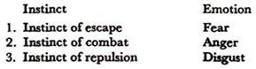
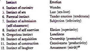
McDougall is right when he enunctates the principle that every emotive situation appeals to an instinctive tendency. But his list based on this principle is unscientific. For example, anger does not always arise from pugnacity; tender emotion may arise from other instincts than the parental.

McDougall mentions a number of instincts with less well-defined emotive reactions, e.g., the instinct of reproduction, the gregarious instinct, the instincts of acquisition and construction. Yet there are well-defined emotions of security, of self-expansion, of possession, etc., which have not been mentioned by McDougall.

His theory is very attractive, but it has not been worked out very satisfactorily. Some instincts (e.g., the instincts of walking, sitting, standing, running, etc.,) seem to have no specific emotions attached to them. Anger and fear resemble each other very closely as organic states, though they differ as impulses.

The really distinct emotions are much fewer than the instincts. So McDougall’s theory may be regarded as a working hypothesis. When we find an emotion, we find also a tendency to action that leads to some end-result.

But though emotion and instinct are closely connected with each other, we cannot hold that corresponding to every instinct there is an emotion and corresponding to every emotion there is an instinct. There are many instincts which are not accompanied by any specific emotions.

Further, the same emotion may include a variety of instinct in its system. The instinct of concealment and flight both operate in the emotion of fear. Again, the same expression may be connected with different emotions. Just as the same emotion may be organized in different sentiments, so the same instinct may be organized in different emotions.

The instinct of flight may operate in birds in fear as well as anger. Moreover, when the instinctive act evoked by a situation runs smoothly, the individual does not feel an emotion. But when the individual cannot effectively cope with the situation and his instinc­tive response is thwarted, he feels an emotion.

Therefore, an in­stinctive act is not always accompanied by an emotion. Hence McDougall’s theory may be regarded as a working hypothesis. It contains core of truth in it; it points out an intimate connection between instinct and emotion.

4. Philips Bard’s Theory of Emotion

Cannon (1927), refuted the James-Lange theory of emotion by showing that experimental subjects experienced and reported emotions before all bodily sensations. Therefore, emotions were not preceded and constituted by bodily sensations.

Bard (1934) later removed the cortex and thalamus of some animals and left only the posterior part of the hypothalamus and found that they still showed rage. But when he removed the hypo­thalamus also, they failed to show the integrated rage pattern.

Thus he proved that the hypothalamus was necessary for the expression of rage. His experiments did not prove that either the thalamus or hypothalamus generated rage (or any other emotion) or did they prove that the cortex normally inhibited the thalamus.

Masserman showed that convincingly by some experiments. He stimulated the hypothalamus in some normal cats by means of bipolar electrodes and they showed the integrated rage pattern, e.g., hissing, spitting, and unsheathing of claws. But these expressions did not disturb their normal activity.

Both Bard and Masserman also obtained the flight reaction in fear in a similar way. Bard removed the cortex and thalamus in cats, who showed fight reaction in response to air-blast. Masserman stimulated the hypothalamus of intact cats and obtained flight reaction.

But fear pattern exhibited by them differed from that of normal animals. Instead of strenuous attempts at escape made by frightened animals, these cats had fits of aimless and hasty running.

5. Emotion of the Ludicrous: Theory of Laughter

We should observe at the outset, that the ludicrous is not identical with the laughable. Laughter may arise from different sources. It may be excited by purely physical stimuli such as tickling. It is of the nature of a reflex action. Laughter may be excited by automatic imitation. You smile at a child and the child will smile at you. The people laugh in a crowd by automatic imitation.

They sometimes do not know the reason why they laugh. Laughter may arise from sympathetic reproduction .of the feelings of others. Emotions have a contagious effect. They spread from one person to another. When others faugh in exuberance of joy, we catch the contagion and laugh.

Laughter may arise from the consciousness of our own superiority over others. When we defeat our powerful adversary, we laugh in excess of elation. Laughter may be excited by the contemplation of the ludicrous.

Thus, the ludicrous is not identical with the laughable. Whatever is ludicrous is laughable, but whatever is laughable is not ludicrous. Laughter has many other causes hand ludicrous objects. The comic, emotion or the emotion of the ludicrous has the following characteristics.

It is an emotion of pure joy or elation unmixed with pain. It has a social significance. It is excited by incongruity in a situation, which is determined by a social standard of propriety or impropriety. It is a disinterested emotion devoid of a utilitarian motive.

Laughter is peculiar to the human species. Man is the only animal that laughs. He does not learn to laugh. He is provided by Nature with the complex mechanism of laughter. The impulse to laugh is instinctive.

Types of Emotions

McDougall classifies emotions into three types:

• Primary emotions
• Secondary or blended emotions
• Derived emotions

1. Primary emotions

Primary emotions are the elementary effective correlates of instincts. Fear, anger, disgust, tender emotion, distress, lust or sex-love, curiosity, amusement, etc., which arise from the instincts of escape, combat, repulsion, parental instinct, appeal, sex, curiosity, laughter, etc., are primary emotions. They do not presuppose other emotions.

2. Secondary or blended emotions

Secondary or blended emotions are the combinations of two or more primary emotions. When two or more cooperating or conflic­ting instinctive impulses are evoked by a complex situation, a secondary or blended emotion is aroused.

It may not be a blend or coalescence of two or more primary emotions. It may arise from a complex situation which excites two or more cooperating or con­flicting instinctive tendencies which generally arouse two or more primary emotions.

It is the immediate response to a complex situation. McDougall avers that his treatment of the secondary emotions is not guilty of the errors of J.S. Mill’s “mental chemistry”. When a child approaches a snake and recedes from it out of fear and curiosity, he feels a blended emotion. Scorn is a blend of anger and disgust. Or, it is a blend of anger, disgust and positive self-feeling or elation.

It is a binary compound or a tertiary compound. Admiration is a compound of wonder and negative self-feeling or self-abasement. Awe is a compound of wonder, self-abasement and fear. Pity is a compound of tender emotion and sympathy pain or distress.

Reproach is a compound of tender feeling and anger. Hate is a blend of anger, fear and disgust. Jealousy, shame, revenge, gratitude, reverence etc., are blended emotions.

3. Derived emotions

Derived emotions are the complex feelings, which are neither primary emotions nor blended motions but which are related to desires. They do not arise from the instinctive impulses. Confidence, hope, anxiety, despondency, despairs, regret, remorse, sorrow, etc., are derivative emotions.

Confidence, hope, anxiety, despondency and despair are the prospective emotions or desire. When a team of mountaineers start on a journey to reach a peak, they have confi­dence due to the anticipation of success. Their confidence arises from a strong desire for success.

When a member of the party falls seriously ill for a certain period, their confidence is reduced to hope. When they are hindered by a series of avalanches and landslides, their hope degenerates into anxiety. When farther on their journey they encounter freezing temperature, and shortage of food, and when some are crippled by frostbite, their anxiety is converted into des­pondency.

Later when their progress is thwarted by foul weather, heavy snowfall, and blizard, their despondency turns into despair. These derived emotions are called by Shand “the prospective emo­tions or desire” because they are related to desire that looks forward to the future.

Regret, remorse, and sorry are derived emotions which are called “the retrospective emotions of desire,” because they are related to desire which looks backward to the past. Regret arises from the frustration of a desire in the past, and is attended with pain.

Regret becomes remorse when the frustration of a desire in the past was due to one’s misjudgement or negligence of duty. It is attended with self-reproach. Sorrow is tender regret arising from the loss of a cherished object. It is a painful emotion of retrospective desire. Derived emotions may arise from prospective or retrospective aversion also.

Primary emotions are based on instincts excited by a situation. Derived emotions are not directly based on instincts, but they pre­suppose some desire or aversion which operates when a situation is apprehended. Primary emotions are comparatively simple and elementary, while derived emotions are complex and presuppose some mental development and operation of prospective or retros­pective desire or aversion.

Development of Emotions

Primary emotions are refined in three ways. First, they are refined by modifications of the motor response by which socially acceptable reactions are substituted for the primitive emotional expressions such as crying, kicking, scratching, biting, etc.

The emotional expressions of a cultured person are different from those of a child or a savage. Secondly, primary emotions are modified by new attachments on the side of the stimulus.

The primary emo­tion of fear is originally excited by the perception of a dangerous situation, e.g., the sight of a tiger at large. But later it is excited by the imagination or thought of a serious situation, e.g., the loss of a job, the imminent death of an earning member of a family, the fall of a Government, etc.

Thirdly, primary emotions are modified by a combination of one with another. Awe is a compound of wonder, fear and humility. Hate is a compound of anger, fear and disgust. Pity is a compound of grief and tenderness”.

The situations which excite specific emotions in older children and adults excite only general excitement in new born infants. Gradually distress, delight, fear, disgust, anger, affection and joy are differentiated from the general excitement in two years.

Maturation and learning both play important roles in the develop­ment of emotion. As the organism matures the infant exhibits such emotional responses as crying, weeping, smiling and laughing without earning them.

They appear almost at the same age in all children even when they are not allowed opportunities to imitate them from others. Facial expressions of deaf-blind children also confirm the influence of maturation in emotional development.

The stereotyped facial and gestural expressions which are peculiar to persons of a particular culture are learned from others. The clapping of hands is a sign of happiness in us, but of disappoint­ment in the Chinese. The raising of the eyebrows and the opening of the eyes widely are expression of surprise in us, but the sticking out of tongues, in them. These peculiar expressions show the in­fluence of learning and culture.

Emotions and their expressions are due to conditioning. A child of nine months exhibited fear reactions to a loud noise. When a rat was placed before him, he had no fear response. But when a rat was placed before him subsequently a number of times when a loud noise was produced on each occasion, the child showed fear reaction. Later when only a rat was placed before him, he exhibited fear reaction.

Thus his fear was conditioned by a substitute stimulus. Sometimes emotions are learned by imitation. If the parent is afraid of particular objects (e.g., darkness, lightning, snakes, etc.), the children get afraid of them. Obviously, their emotion is influenced by imitation.

Degrees of Emotional Responsiveness

Normal persons differ in their general emotional responsiveness. There are calm persons who are generally not perturbed, by emo­tions. There are excitable persons who are deeply stirred by emo­tions. These are two extremes. There are many degrees of emo­tionality between these two extremes.

1. Emotional Excess

Some persons have an excess of emo­tionally. They are susceptible to all emotions. Their emotions are easily excited by slight stimuli. Joy, fear, anger, sorrow, and other emotions are easily and frequently aroused. They are usually intense. Joy becomes ecstasy, fear becomes terror, anger becomes violent rage, and sorrow becomes’ intense grief. Emotions are felt in their intensity.

2. Emotionally Instability

Generally the persons who have an excess of emotionality have also emotional instability. They often shift abruptly from joy to sorrow, from love to hate; from self-confidence to diffidence. This is called emotional instability. It is generally accompanied by emotional sensitivity and excess of response.

But excessive emotionality and emotional instability do not invariably go together. Sometimes emotional instability is found along with nervous and mental instability.

3. Unemotional Nature

The extremely unemotional individual is not dead to all emotions. But his emotions are not easily aroused. They are by no means unemotional. Unemotional persons do not experience difficulties in adapting themselves to the social environ­ment. But over-emotional persons cannot easily adapt themselves to it.

In the emotional person the sympathetic nervous system is readily excited and brings about visceral changes. Excessive sensi­tivity of the sympathetic systems is the cause of excessive emotionality and emotional instability.

The term “thinking skills” refers to the specific mental and cognitive processes that a person draws upon to think effectively. Basically, thinking skills are what we use in our heads to problem-solve, reason, infer and hypothesize.

Thinking skills are the mental activities you use to process information, make connections, make decisions, and create new ideas. You use your thinking skills when you try to make sense of experiences, solve problems, make decisions, ask questions, make plans, or organize information.

Types of Thinking Skills

The 4 types of thinking skills are:

1. Convergent Analytical Thinking

Convergent thinking is the process of coming up with the best answer to a question using our memory, resources around us, or logic.

This thinking skill does not require significant creativity or lateral thinking strategies. Instead, it uses very straightforward thought processes. A convergent thinker simply needs to apply already established procedures and memory recall to reach the ‘correct’ answer.

Convergent thinking is very commonly used for standardized and multiple choice tests. These sorts of tests simply assess our knowledge and ability to apply knowledge to simple and logical situations.

The key elements required to be a skilled convergent thinker are: speed, accuracy and logic.

2. Divergent Thinking

Divergent thinking is the exact opposite of convergent thinking. It involves coming up to solutions, paths forward or new ideas when there is no single correct answer. Questions like “should I study to become a doctor or a lawyer?” may not have a simple answer. You might be good at both, and both options might bring you happiness and a good life. So, which option should you choose?

To come up with solutions to questions without clear answers, you need to break down the possibilities and analyze each part. You might create a pros and cons list, a venn diagram or a table to lay out your options and consider each one in turn.

We often encourage divergent thinking from a very young age. For example, we encourage children to play or simply ‘be playful’ in order to discover how their world is complex and full of possibility.

3. Critical Thinking

Critical thinking involves analyzing something in order to form a judgement about it. A critical thinker does not take the assumptions of a topic for granted. Instead, the thinkers ‘critiques’ what they are viewing using their available intellectual knowledge.

Critical thinkers can use three processes to develop critical insights on a topic: deduction, induction and abduction.

Deduction is the process of drawing conclusions based on the facts at hand. You have all the facts available to you to come to a clear and unambiguous conclusion about a topic. For example, a doctor does blood tests to determine if someone has a virus. The blood tests come back positive, so we can deduce that you definitely have that virus.

Induction is the process of drawing conclusions based on a generalization. You don’t have all the exact information at hand. However, you are aware of patterns, clues and a methodology that can help you induce the answer For example, you come to the doctor exhibiting a fever, sneezing and coughing. The doctor doesn’t do tests, but they induce that you probably have influenza because your symptoms are characteristic of someone with the flu.

Abduction involves coming to a conclusion that is the most likely or logical based on the small amount of knowledge that you have. You can’t be sure of the answer, but you can guess. For example, you may see that a cat is on the roof. The most logical answer is that the cat got up there by climbing a nearby tree and jumping from it to the roof, but you can’t be sure.

4. Creative Thinking

Creative thinking involves thinking about a topic in unusual, unconventional and alternative ways to generate new ideas about an established topic. A creative thinker will try to address an issue from a perspective that hasn’t been used before.

While creative thinking may appear illogical, it is in fact a great driver of human development. Creative thinkers identify gaps in marketplaces or new, easier, faster and better ways of doing things. When a creative thinker comes up with a great new way of approaching an issue, their new method can become the new orthodoxy.

How to Improve your Thinking Skills?

To improve your thinking skills, you need to go beyond just maintaining your mind. You cannot just keep doing the same thing day-in, day-out and expect to get better.

Instead, you need to exercise new parts of your brain by studying regularly and keep creating new neural pathways in your mind. This emphasizes the importance of education.

You always need to be thinking about things that are new and difficult for you to understand.

The things that you learn need to be difficult. It’s through the difficulty and discomfort in thinking that you are improving your thinking. It’s just like going to the gym: no pain, no gain.

Some ways to improve your thinking include:

• Taking college courses (or one of these alternatives) in topics that you find very difficult
• Taking classes in an online school
• Learning using new learning strategies that make you uncomfortable
• Taking up new and diverse hobbies

The more you think, the better you will get at thinking. You’ll become faster, more creative and overall better at thinking if you practice and try out new strategies.

Tools to Help you Think Better

There are also some tools that we call cognitive tools that help you with your thinking skills. These tools don’t do the thinking for you, but they help you with your thinking.

Thinking tools can help you think better by:

• Helping you structure your thoughts
• Giving you a blueprint or scaffold for finding new angles to approach a topic
• Providing prompts to move your thinking forward

Some tools that can help you think better include:

1. A Brainstorming Mind Map

A brainstorming mind map can be made with a simple piece of paper. Simply write the topic at the top of the piece of paper and scrawl any and all key things you can think about down onto the paper.

During the brainstorming process, no ideas are bad ideas. You can critique and dismiss some of your ideas later on; but the brainstorming session can help get your mind moving.

2. A Radar Chart

A radar (or spider) chart is very similar to a brainstorming mind map, but it also shows the links between concepts.

To create a spider chart, write the topic you’re thinking about in the middle of the piece of paper.

When you come up with a new idea, write it near the middle of the paper and draw a line from the topic in the center to the idea. If you come up with new ideas or sub-ideas based on that first key idea, you can write them down and draw a line from one idea to the other. Whenever you come up with related ideas, you should draw a line between them to show their relationship.

3. A Process Chart

A process chart shows the sequence of steps from a question to its logical answer. Often in science and mathematics classes, you need to provide your process chart to your teacher to show how you came to your conclusions. You may hear your teacher tell you to “show your thinking”!

4. A Spreadsheet

Even a simple spreadsheet using Excel or Google Sheets can help with your thinking. It will help you lay out ideas into an easy-to-read table to help you keep track of your thoughts, your processes and your different categories. Categorizing ideas into columns and rows can help you to identify new patterns in data.

5. A Pros and Cons List

A simple pros and cons list can help you to get your ideas out of your brain and onto paper. Once it’s on paper, you can go through the list systematically and compare the pros and cons directly with one another. Once you’ve done this, you may have a better idea of what conclusions to come to.

6. De Bono’s Six Thinking Hats

Another strategy for helping your thinking is to use De Bono’s Six Thinking Hats. These are six metaphorical ‘hats’ that you can put on. Each hat represents a different way to look at a topic. When you ‘put the hat on’, you have to think from the perspective of the hat.

The six hats are:

• Red Hat: Think about your feelings, emotions and hunches about a topic
• White Hat: Think about the information that’s available to you and what it can reveal about the topic
• Yellow Hat: Think about the benefits and value in the situation you’re thinking about.
• Black Hat: Think about the risks, difficulties and challenges that a situation you’re thinking about may cause.
• Green Hat: Think about the alternatives and creative approaches you can apply to a topic.
• Blue Hat: Think about the processes you can use and how to manage the situation logically.

“Thinking is more interesting than knowing, but less interesting than looking” :Johann Wolfgang von Goethe

You improve your communication with others when you can match their thinking style.

You can also avoid rubbing your boss the wrong way by paying close attention to how they approach the tasks of the day.

In Coping with Difficult Bosses, Robert Bramson identifies five thinking styles to categorize our modes of thinking and problem solving we use most frequently.

Five Thinking Styles

According to Bramson, the five thinking styles are:

1. Synthesists

According to Bramson, “Synthesists are creative thinkers who perceives the world in terms of opposites.  When you say black, they think white, when you say long, they think short.”

To connect with Synthesists, Bramson suggests “listen appreciatively to their speculation and don’t confuse their arguing nature with resistance.”

2. Idealists

According to Bramson, “Idealists believe in lofty goals and standards.”

To connect with Idealists, Bramson suggests “associate what you want to do with these goals of quality, service, and community good.”

3. Pragmatic Thinkers

According to Bramson, “Pragmatic thinkers are flexible, resourceful folk who look for immediate payoff rather than for a grand plan that will change the world.”

To connect with Pragmatists, Bramson suggests “emphasize short-term objectives on which you can get started with resources at hand.”

4. Analyst Thinkers

 According to Bramsom, “Analyst thinkers equate accuracy, thoroughness, and attention to detail with completeness.  They are likely to gather data, measure it, categorize it, and rationally and methodically calculate the right answer to any problem you come up with.

To connect to Analysts, Bramson suggests “provide a logical plan replete with back-up data and specifications.”

5. Realist Thinkers

According to Bramson, “Realist thinkers are fast moving doers who know that reality is what their senses sight, sound, taste, smell, and touch tell them it is, and not that dry stuff that one finds in accounting ledgers, or the insipid pages of manual of operations.”

To connect with Realists, Bramson suggests focus on the challenge and your solution.

“If you communicate with Realist bosses as if they were Analysts, you will never get their attention. Rather than gobs of computer-printouts and other detailed information, Realists want a three-paragraph ‘Executive Summary’ which tells briefly what is wrong and how you propose to fix it. For rather complicated reasons, they will often take you at your word if they see you as a qualified expert. You become an expert in their eyes when they know that you’ve assembled a store of facts in which they are interested, and you have proposed a set of actions that they already believe are the best things to do.”

How to Use the Five Thinking Styles?

Take the time to place your boss or who you need to interact with into one or two of the five thinking-style categories. Keep in mind that while one or two styles predominates for most people, about fifteen percent use all five styles equally. Those who do, are seldom difficult bosses. Once you’ve identified their preferred categories, figure out how you can change your approach to better suit their style.

Here are my key take aways:

• Seek first to understand, then to be understood. The more you understand somebody, the better you can adapt your style. I think the five thinking styles are a helpful framework in addition to understanding somebody’s learning style ( auditory, visual, or kinesthtic), their NLP meta-programs, their motivation (towards pleasure or away from pain), their values, their “rules”, their extraversion and introversion tendencies, their passive or aggressive tendencies, whether they are more “task-centered” or “people-centered”, their decision making style (consult-and-decide or build consensus), and their management styles (Autocratic, Paternalistic, Democratic, and Laissez-faire.)
• Establish rapport. I think the heart of identifying the five thinking-styles revolves around establishing rapport. Rapport is the key to communication, influence, and trust.
• Know the anti-patterns. It’s probably more important to know how to avoid rubbing somebody the wrong way, than getting the preferred or ideal communication style exactly right.
• Wear different hats. I think you can use the Six-Thinking Hats concept to switch your hat based on who you are working with. Each hat you put on or take off can represent a different thinking style

A little insight can go a long way when it comes to connecting with people.

If you can bridge the gap between their thinking style and yours, you’ll have more rapport and get better results.

Six Thinking Hats was created by Edward de Bono, and published in his 1985 book of the same name.

It forces you to move outside your habitual thinking style, and to look at things from a number of different perspectives. This allows you to get a more rounded view of your situation.

You can often reach a successful solution or outcome from a rational, positive viewpoint, but it can also pay to consider a problem from other angles. For example, you can look at it from an emotional, intuitive, creative or risk management viewpoint. Not considering these perspectives could lead you to underestimate people’s resistance to your plans, fail to make creative leaps, or ignore the need for essential contingency plans.

You can use Six Thinking Hats in meetings or on your own. In meetings, it has the benefit of preventing any confrontation that may happen when people with different thinking styles discuss a problem, because every perspective is valid.

Each “Thinking Hat” is a different style of thinking. These are explained below:

1. White Hat

With this thinking hat, you focus on the available data. Look at the information that you have, analyze past trends, and see what you can learn from it. Look for gaps in your knowledge, and try to either fill them or take account of them.

2. Red Hat

“Wearing” the Red Hat, you look at problems using your intuition, gut reaction, and emotion. Also, think how others could react emotionally. Try to understand the responses of people who do not fully know your reasoning.

3. Black Hat

Using Black Hat thinking, look at a decision’s potentially negative outcomes. Look at it cautiously and defensively. Try to see why it might not work. This is important because it highlights the weak points in a plan. It allows you to eliminate them, alter them, or prepare contingency plans to counter them.

Black Hat thinking helps to make your plans “tougher” and more resilient. It can also help you to spot fatal flaws and risks before you embark on a course of action. It’s one of the real benefits of this model, as many successful people get so used to thinking positively that they often cannot see problems in advance. This leaves them under-prepared for difficulties.

4. Yellow Hat

This hat helps you to think positively. It is the optimistic viewpoint that helps you to see all the benefits of the decision and the value in it. Yellow Hat thinking helps you to keep going when everything looks gloomy and difficult.

5. Green Hat

The Green Hat represents creativity. This is where you develop creative solutions to a problem. It is a freewheeling way of thinking, in which there is little criticism of ideas. (You can explore a range of creativity tools to help you.)

6. Blue Hat

This hat represents process control. It’s the hat worn by people chairing meetings, for example. When facing difficulties because ideas are running dry, they may direct activity into Green Hat thinking. When contingency plans are needed, they will ask for Black Hat thinking.

A variant of this technique is to look at problems from the point of view of different professionals (for example, doctors, architects or sales directors) or different customers.

An Example of Six Hat Thinking

The directors of a property company are considering whether they should build a new office block. The economy is doing well, and the vacant office spaces in their city are being snapped up. As part of their decision-making process, they adopt the Six Thinking Hats technique.

Wearing the White Hat, they analyze the data that they have. They can see that the amount of available office space in their city is dwindling, and they calculate that, by the time a new office block would be completed, existing space will be in extremely short supply. They also note that the economic outlook is good, and steady growth is predicted to continue.

Thinking with a Red Hat, some of the directors say that the proposed building looks ugly and gloomy. They worry that people would find it an oppressive or uninspiring place to work.

When they think with the Black Hat, they wonder whether the economic forecast could be wrong. The economy may be about to experience a downturn, in which case the building could sit empty or only partially occupied for a long time. If the building is unattractive, then companies will choose to work in other, more attractive premises.

Wearing the positive Yellow Hat, however, the directors know that, if the economy holds up and their projections are correct, the company stands to make a healthy profit. If they are lucky, maybe they could sell the building before the next downturn, or rent to tenants on long-term leases that will last through any recession.

With Green Hat thinking, they consider whether they should redesign the building to make it more appealing. Perhaps they could build prestige offices that people would want to rent in any economic climate. Alternatively, maybe they should invest the money in the short term, then buy up property at a lower cost when the next downturn happens.

The chairman of the meeting wears the Blue Hat to keep the discussion moving and ideas flowing, encouraging the other directors to switch their thinking between the different perspectives.

Having examined their options from numerous viewpoints, the directors have a much more detailed picture of possible outcomes, and can make their decision accordingly.