Tag: Entry Barriers

Indifference curve analysis is basically an attempt to improve cardinal utility analysis (principle of marginal utility). The cardinal utility approach, though very useful in studying elementary consumer behavior, is criticized for its unrealistic assumptions vehemently. In particular, economists such as Edgeworth, Hicks, Allen and Slutsky opposed utility as a measurable entity. According to them, utility is a subjective phenomenon and can never be measured on an absolute scale. The disbelief on the measurement of utility forced them to explore an alternative approach to study consumer behavior. The exploration led them to come up with the ordinal utility approach or indifference curve analysis. Because of this reason, aforementioned economists are known as ordinalists. As per indifference curve analysis, utility is not a measurable entity. However, consumers can rank their preferences.

Indifference Curve Analysis Vs. Marginal Utility Approach

Let us look at a simple example. Suppose there are two commodities, namely apple and orange. The consumer has $10. If he spends entire money on buying apple, it means that apple gives him more satisfaction than orange. Thus, in indifference curve analysis, we conclude that the consumer prefers apple to orange. In other words, he ranks apple first and orange second. However, in cardinal or marginal utility approach, the utility derived from apple is measured (for example, 10 utils). Similarly, the utility derived from orange is measured (for example, 5 utils). Now the consumer compares both and prefers the commodity that gives higher amount of utility. Indifference curve analysis strictly says that utility is not a measurable entity. What we do here is that we observe what the consumer prefers and conclude that the preferred commodity (apple in our example) gives him more satisfaction. We never try to answer ‘how much satisfaction (utility)’ in indifference curve analysis.

Assumptions

Theories of economics cannot survive without assumptions and indifference curve analysis is no different. The following are the assumptions of indifference curve analysis:

• Rationality

The theory of indifference curve studies consumer behavior. In order to derive a plausible conclusion, the consumer under consideration must be a rational human being. For example, there are two commodities called ‘A’ and ‘B’. Now the consumer must be able to say which commodity he prefers. The answer must be a definite. For instance – ‘I prefer A to B’ or ‘I prefer B to A’ or ‘I prefer both equally’. Technically, this assumption is known as completeness or trichotomy assumption.

• Consistency

Another important assumption is consistency. It means that the consumer must be consistent in his preferences. For example, let us consider three different commodities called ‘A’, ‘B’ and ‘C’. If the consumer prefers A to B and B to C, obviously, he must prefer A to C. In this case, he must not be in a position to prefer C to A since this decision becomes self-contradictory.

Symbolically,

If A > B, and B > c, then A > C.

• More Goods to Less

The indifference curve analysis assumes that consumer always prefers more goods to less. Suppose there are two bundles of commodities – ‘A’ and ‘B’. If bundle A has more goods than bundle B, then the consumer prefers bundle A to B.

• Substitutes and Complements

In indifference curve analysis, there exist substitutes and complements for the goods preferred by the consumer. However, in marginal utility approach, we assume that goods under consideration do not have substitutes and complements.

• Income and Market Prices

Finally, the consumer’s income and prices of commodities are fixed. In other words, with given income and market prices, the consumer tries to maximize utility.

• Indifference Schedule

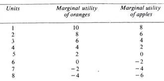
An indifference schedule is a list of various combinations of commodities that give equal satisfaction or utility to consumers. For simplicity, we have considered only two commodities, ‘X’ and ‘Y’, in our Table 1. Table 1 shows various combinations of X and Y; however, all these combinations give equal satisfaction (k) to the consumer.

Table 1: Indifference Schedule

Combinations	X (Oranges)	Y (Apples)	Satisfaction
A	2	15	k
B	5	9	k
C	7	6	k
D	17	2	k

You can construct an indifference curve from an indifference schedule in the same way you construct a demand curve from a demand schedule.

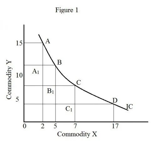
On the graph, the locus of all combinations of commodities (X and Y in our example) forms an indifference curve (figure 1). Movement along the indifference curve gives various combinations of commodities (X and Y); however, yields same level of satisfaction. An indifference curve is also known as iso utility curve (“iso” means same). A set of indifference curves is known as an indifference map.

Marginal Rate of Substitution

Marginal rate of substitution is an eminent concept in the indifference curve analysis. Marginal rate of substitution tells you the amount of one commodity the consumer is willing to give up for an additional unit of another commodity. In our example (table 1), we have considered commodity X and Y. Hence, the marginal rate of substitution of X for Y (MRS_xy) is the maximum amount of Y the consumer is willing to give up for an additional unit of X. However, the consumer remains on the same indifference curve.

In other words, the marginal rate of substitution explains the tradeoff between two goods.

Diminishing marginal rate of substitution

From table 1 and figure 1, we can easily explain the concept of diminishing marginal rate of substitution. In our example, we substitute commodity X for commodity Y. Hence, the change in Y is negative (i.e., -ΔY) since Y decreases.

Thus, the equation is

MRS_xy = -ΔY/ΔX and

MRS_yx = -ΔX/ΔY

However, convention is to ignore the minus sign; hence,

MRS_xy = ΔY/ΔX

In figure 1, X denotes oranges and Y denotes apples. Points A, B, C and D indicate various combinations of oranges and apples.

In this example, we have the following marginal rate of substitution:

MRS_{x for y} between A and B: AA_­­1/A₁B = 6/3 = 2.0

MRS_{x for y} between B and C: BB_­­1/B₁C = 3/2 = 1.5

MRS_{x for y} between C and D: CC_­­1/C₁D = 4/10 = 0.4

Thus, MRS_{x for y} diminishes for every additional units of X. This is the principle of diminishing marginal rate of substitution.

Law of Diminishing Marginal Utility states that as a person consumes additional units of a good or service, the satisfaction (utility) derived from each successive unit decreases, assuming all other factors remain constant. Initially, the first few units provide significant satisfaction, but as consumption increases, the utility of each extra unit diminishes. For example, the first slice of pizza may bring great joy, but by the fifth or sixth slice, the additional satisfaction reduces. This principle underlies consumer behavior and helps explain demand curves, as consumers are less willing to pay the same price for additional units of a product.

Assumptions:

Following are the assumptions of the law of diminishing marginal utility.

1. The utility is measurable and a person can express the utility derived from a commodity in qualitative terms such as 2 units, 4 units and 7 units etc.
2. A rational consumer aims at the maximization of his utility.
3. It is necessary that a standard unit of measurement is constant
4. A commodity is being taken continuously. Any gap between the consumption of a commodity should be suitable.
5. There should be proper units of a good consumed by the consumer.
6. It is assumed that various units of commodity homogeneous in characteristics.
7. The taste of the consumer remains same during the consumption o the successive units of commodity.
8. Income of the consumer remains constant during the operation of the law of diminishing marginal utility.
9. It is assumed that the commodity is divisible.

• There should be not change in fashion. For example, if there is a fashion of lifted shirts, then the consumer may have no utility in open shirts.
• It is assumed that the prices of the substitutes do not change. For example, the demand for CNG increases due to rise in the prices of petroleum and these price changes effect the utility of CNG.

Explanation with Schedule and Diagram:

We assume that a man is very thirsty. He takes the glasses of water successively. The marginal utility of the successive glasses of water decreases, ultimately, he reaches the point of satiety. After this point the marginal utility becomes negative, if he is forced further to take a glass of water. The behavior of the consumer is indicated in the following schedule:

Units of commodity	Marginal utility	Total utility
1st glass	10	10
2nd glass	8	18
3rd glass	6	24
4th glass	4	28
5th glass	2	30
6th glass	0	30
7th glass	-2	28

On taking the 1st glass of water, the consumer gets 10 units of utility, because he is very thirsty. When he takes 2nd glass of water, his marginal utility goes down to 8 units because his thirst has been partly satisfied. This process continues until the marginal utility drops down to zero which is the saturation point. By taking the seventh glass of water, the marginal utility becomes negative because the thirst of the consumer has already been fully satisfied.

The law of diminishing marginal utility can be explained by the following diagram drawn with the help of above schedule:

In the above figure, the marginal utility of different glasses of water is measured on the y-axis and the units (glasses of water) on X-axis. With the help of the schedule, the points A, B, C, D, E, F and G are derived by the different combinations of units of the commodity (glasses of water) and the marginal utility gained by different units of commodity. By joining these points, we get the marginal utility curve. The marginal utility curve has the downward negative slope. It intersects the X-axis at the point of 6th unit of the commodity. At this point “F” the marginal utility becomes zero. When the MU curve goes beyond this point, the MU becomes negative. So there is an inverse functional relationship between the units of a commodity and the marginal utility of that commodity.

Exceptions or Limitations:

The limitations or exceptions of the law of diminishing marginal utility are as follows:

1. The law does not hold well in the rare collections. For example, collection of ancient coins, stamps etc.
2. The law is not fully applicable to money. The marginal utility of money declines with richness but never falls to zero.
3. It does not apply to the knowledge, art and innovations.
4. The law is not applicable for precious goods.
5. Historical things are also included in exceptions to the law.
6. Law does not operate if consumer behaves in irrational manner. For example, drunkard is said to enjoy each successive peg more than the previous one.
7. Man is fond of beauty and decoration. He gets more satisfaction by getting the above merits of the commodities.
8. If a dress comes in fashion, its utility goes up. On the other hand its utility goes down if it goes out of fashion.
9. The utility increases due to demonstration. It is a natural element.

Importance of the Law of Diminishing Marginal Utility:

1. By purchasing more of a commodity the marginal utility decreases. Due to this behaviour, the consumer cuts his expenditures to that commodity.
2. In the field of public finance, this law has a practical application, imposing a heavier burden on the rich people.
3. This law is the base of some other economic laws such as law of demand, elasticity of demand, consumer surplus and the law of substitution etc.

4. The value of commodity falls by increasing the supply of a commodity. It forms a basis of the theory of value. In this way prices are determined

Equi-Marginal Principle (also known as the principle of equal marginal utility or the law of equi-marginal utility) is a fundamental concept in economics that helps individuals and businesses maximize satisfaction or profit. According to this principle, resources should be allocated in such a way that the marginal utility or marginal returns from each resource are equal across all possible uses.

In other words, whether a consumer is trying to maximize their utility or a firm is trying to maximize profit, they will distribute their limited resources (money, labor, time, etc.) among various alternatives so that the additional (marginal) benefit derived from the last unit of resource used in each alternative is equal.

Key Elements of the Equi-Marginal Principle:

1. Marginal Utility:

Marginal utility refers to the additional satisfaction or benefit that a person receives from consuming an additional unit of a good or service. As more of a good is consumed, the marginal utility usually decreases, a concept known as diminishing marginal utility.

2. Marginal Productivity/Returns:

In business, marginal productivity or marginal returns refer to the additional output that can be obtained by using an additional unit of input. Like marginal utility, marginal returns also generally diminish as more units of input are added.

3. Optimization:

The equi-marginal principle is about optimization. Consumers aim to allocate their resources (income) in such a way that the marginal utility per unit of money spent is equal for all goods. Similarly, firms allocate inputs like labor and capital to maximize profit, ensuring that the marginal returns from each input are equal across all uses.

Formula for the Equi-Marginal Principle

For consumers: The formula for maximizing utility using the equi-marginal principle is as follows:

Example: Allocation of Consumer Budget

Let’s assume a consumer has a budget of $100 to spend on two goods, A and B. The consumer’s goal is to allocate their budget in such a way that the total utility derived from consuming both goods is maximized.

Table of Marginal Utility and Price:

Units Consumed	Marginal Utility of A (MUA​)	Price of A (PA​)	MUA​/PA​	Marginal Utility of B (MUB​)	Price of B (PB​)	MUB​/PB​
1	20	$10	2	24	$8	3
2	18	$10	1.8	20	$8	2.5
3	16	$10	1.6	16	$8	2
4	14	$10	1.4	12	$8	1.5
5	12	$10	1.2	8	$8	1

From the table, we can see the marginal utility per dollar spent on each good for various levels of consumption.

Allocation Process:

1. Initially, the consumer will compare the MU/P ratios for both goods.
2. The consumer will spend their first dollar on Good B because it provides a higher marginal utility per dollar (3) than Good A (2).
3. After consuming the first unit of Good B, the consumer will compare the MU/P ratios again. Since MUB/PB=2.5 is still higher than MUA/PA=2, the consumer will purchase another unit of Good B.
4. This process will continue until the MU/P ratios for both goods are equal or the consumer’s budget is exhausted.

In this case, the consumer might end up purchasing 2 units of Good A and 3 units of Good B, at which point the marginal utility per dollar for both goods becomes approximately equal, maximizing their total utility.

Example: Firm’s Input Allocation

Let’s assume a firm has two inputs: labor (L) and capital (K). The firm wants to allocate these inputs to maximize profit, with the marginal product and cost data as follows:

Input	Marginal Product of Labor (MPL​)	Cost of Labor (CL)	MPL​/CL​	Marginal Product of Capital (MPK​)	Cost of Capital (CK​)	MPK​/CK​
1	50	$10	5	80	$20	4
2	40	$10	4	70	$20	3.5
3	30	$10	3	60	$20	3
4	20	$10	2	50	$20	2.5
5	10	$10	1	40	$20	2

The firm’s goal is to allocate labor and capital in such a way that the marginal product per unit of cost is equal for both inputs.

Allocation Process:

1. Initially, the firm compares the MP/C ratios for labor and capital.
2. The firm will allocate its first dollar towards labor, where MPL/CL=5 is greater than MPK/CK=4.
3. After allocating more resources, the firm will continue comparing the ratios.
4. The firm will keep allocating resources until the marginal product per unit cost for both labor and capital is equal.

In this case, the optimal allocation would involve using 2 units of labor and 1 unit of capital, where the marginal products per unit cost are equal (4), maximizing the firm’s profit.

Importance of the Equi-Marginal Principle:

• Efficient Allocation:

The equi-marginal principle ensures the efficient allocation of resources, whether for consumers aiming to maximize utility or firms aiming to maximize profit. By allocating resources where they provide the highest marginal benefit, both individuals and businesses can make the best possible use of their limited resources.

• Economic Decision-Making:

This principle is a key component of rational decision-making in economics. It helps in determining the optimal quantity of goods to consume, the best mix of inputs to use in production, or even the best way to allocate time among different activities.

• Flexibility:

The equi-marginal principle can be applied across various fields of economics, from consumer theory and production theory to cost minimization and utility maximization.

Explanation of the Law:

In order to get maximum satisfaction out of the funds we have, we carefully weigh the satisfaction obtained from each rupee ‘had we spend If we find that a rupee spent in one direction has greater utility than in another, we shall go on spending money on the former commodity, till the satisfaction derived from the last rupee spent in the two cases is equal.

It other words, we substitute some units of the commodity of greater utility tor some units of the commodity of less utility. The result of this substitution will be that the marginal utility of the former will fall and that of the latter will rise, till the two marginal utilities are equalized. That is why the law is also called the Law of Substitution or the Law of equimarginal Utility.

Suppose apples and oranges are the two commodities to be purchased. Suppose further that we have got seven rupees to spend. Let us spend three rupees on oranges and four rupees on apples. What is the result? The utility of the 3rd unit of oranges is 6 and that of the 4th unit of apples is 2. As the marginal utility of oranges is higher, we should buy more of oranges and less of apples. Let us substitute one orange for one apple so that we buy four oranges and three apples.

Now the marginal utility of both oranges and apples is the same, i.e., 4. This arrangement yields maximum satisfaction. The total utility of 4 oranges would be 10 + 8 + 6 + 4 = 28 and of three apples 8 + 6 + 4= 18 which gives us a total utility of 46. The satisfaction given by 4 oranges and 3 apples at one rupee each is greater than could be obtained by any other combination of apples and oranges. In no other case does this utility amount to 46. We may take some other combinations and see.

We thus come to the conclusion that we obtain maximum satisfaction when we equalize marginal utilities by substituting some units of the more useful for the less useful commodity. We can illustrate this principle with the help of a diagram.

Diagrammatic Representation:

In the two figures given below, OX and OY are the two axes. On X-axis OX are represented the units of money and on the Y-axis marginal utilities. Suppose a person has 7 rupees to spend on apples and oranges whose diminishing marginal utilities are shown by the two curves AP and OR respectively.

The consumer will gain maximum satisfaction if he spends OM money (3 rupees) on apples and OM’ money (4 rupees) on oranges because in this situation the marginal utilities of the two are equal (PM = P’M’). Any other combination will give less total satisfaction.

Let the purchase spend MN money (one rupee) more on apples and the same amount of money, N’M'( = MN) less on oranges. The diagram shows a loss of utility represented by the shaded area LN’M’P’ and a gain of PMNE utility. As MN = N’M’ and PM=P’M’, it is proved that the area LN’M’P’ (loss of utility from reduced consumption of oranges) is bigger than PMNE (gain of utility from increased consumption of apples). Hence the total utility of this new combination is less.

We then, conclude that no other combination of apples and oranges gives as great a satisfaction to the consumer as when PM = P’M’, i.e., where the marginal utilities of apples and oranges purchased are equal, with given amour, of money at our disposal.

Limitations of the Law of Equi-marginal Utility

Like other economic laws, the law of equimarginal utility too has certain limitations or exceptions. The following are the main exception.

(i) Ignorance

If the consumer is ignorant or blindly follows custom or fashion, he will make a wrong use of money. On account of his ignorance he may not know where the utility is greater and where less. Thus, ignorance may prevent him from making a rational use of money. Hence, his satisfaction may not be the maximum, because the marginal utilities from his expenditure can­not be equalised due to ignorance.

(ii) Inefficient Organisation

In the same manner, an incompetent organ­iser of business will fail to achieve the best results from the units of land, labour and capital that he employs. This is so because he may not be able to divert expenditure to more profitable channels from the less profitable ones.

(iii) Unlimited Resources

The law has obviously no place where this resources are unlimited, as for example, is the case with the free gifts of nature. In such cases, there is no need of diverting expenditure from one direction to another.

(iv) Hold of Custom and Fashion

A consumer may be in the strong clutches of custom, or is inclined to be a slave of fashion. In that case, he will not be able to derive maximum satisfaction out of his expenditure, because he cannot give up the consumption of such commodities. This is specially true of the conventional necessaries like dress or when a man is addicted to some into­xicant.

(v) Frequent Changes in Prices

Frequent changes in prices of different goods render the observance of the law very difficult. The consumer may not be able to make the necessary adjustments in his expenditure in a constantly changing price situation.

Micro Economics

Microeconomics studies the behavior and decision-making processes of individual consumers and firms. It focuses on how they allocate scarce resources to maximize utility and profit, respectively. Key concepts include supply and demand, market equilibrium, elasticity, and marginal analysis. Microeconomics examines how factors such as price changes, consumer preferences, and production costs affect the choices of buyers and sellers. It also explores market structures—like perfect competition, monopoly, and oligopoly—and their impact on pricing and output. By analyzing these components, microeconomics helps understand how markets function and how individual decisions influence economic outcomes.

Features of Micro Economics:

1. Individual Decision-Making

Microeconomics centers on how individuals and firms make choices regarding the allocation of their limited resources. It examines consumer behavior, including how preferences and budget constraints influence purchasing decisions, and firm behavior, focusing on production choices and cost management. This feature helps understand the rationale behind personal and business decisions.

2. Supply and Demand Analysis

A fundamental feature of microeconomics is the study of supply and demand. It explores how these forces interact to determine prices and quantities in individual markets. Demand refers to consumer willingness and ability to purchase goods, while supply pertains to the quantity producers are willing to offer. The equilibrium point, where supply equals demand, is crucial for understanding market dynamics.

3. Price Mechanism

Microeconomics investigates how prices are determined in various market structures. It looks at how changes in supply and demand affect prices and how prices signal to producers and consumers about resource allocation. The price mechanism helps in understanding how markets clear and how resources are efficiently allocated based on market signals.

4. Elasticity

Elasticity measures how sensitive the quantity demanded or supplied of a good is to changes in price or other factors. Microeconomics studies price elasticity of demand, income elasticity, and cross-price elasticity, which helps determine how changes in prices, consumer income, or the prices of related goods affect market behavior.

5. Market Structures

Microeconomics analyzes different market structures, including perfect competition, monopoly, monopolistic competition, and oligopoly. Each structure has unique characteristics regarding the number of firms, product differentiation, and pricing power. Understanding these structures helps explain variations in market outcomes and competitive strategies.

6. Marginal Analysis

Marginal analysis is a key feature where decisions are made based on marginal changes. It involves examining the additional benefit (marginal benefit) and additional cost (marginal cost) of a decision to determine the optimal level of production or consumption. This analysis helps in maximizing profit or utility.

7. Consumer Theory

Consumer theory explores how individuals make consumption choices to maximize their utility given their budget constraints. It involves analyzing indifference curves and budget constraints to understand how consumers allocate their income among various goods and services to achieve the highest satisfaction.

8. Production and Costs

Microeconomics examines how firms produce goods and services and the associated costs. It includes the study of production functions, which describe the relationship between input factors and output, and cost structures, such as fixed and variable costs. This feature helps in understanding how firms optimize production and manage costs to maximize profit.

Macro Economics

Macroeconomics examines the economy as a whole, focusing on aggregate phenomena and large-scale economic factors. Key concepts include Gross Domestic Product (GDP), inflation, unemployment, and national income. It explores how these aggregate variables interact and influence each other, and assesses the overall health and performance of an economy. Macroeconomics also studies fiscal and monetary policies—such as government spending, taxation, and central bank interest rates—and their impact on economic growth, stability, and employment. By analyzing these broad economic indicators, macroeconomics aims to understand and manage economic fluctuations and promote overall economic well-being.

Features of Macro Economics:

1. Aggregate Indicators

Macroeconomics examines aggregate indicators such as Gross Domestic Product (GDP), inflation rate, unemployment rate, and national income. These indicators provide a comprehensive view of the overall economic performance and health, helping policymakers and economists understand economic trends and conditions.

2. Economic Growth

A central focus of macroeconomics is understanding and promoting economic growth. It analyzes factors that contribute to increases in a country’s productive capacity over time, such as technological advancements, capital accumulation, and improvements in labor productivity. Economic growth is crucial for improving living standards and fostering long-term prosperity.

3. Business Cycles

Macroeconomics studies business cycles, which are the fluctuations in economic activity over time, characterized by periods of expansion and contraction. It investigates the causes and effects of these cycles, including their impact on employment, investment, and economic output. Understanding business cycles helps in forecasting economic conditions and formulating stabilization policies.

4. Monetary Policy

Monetary policy is a key aspect of macroeconomics, involving the management of the money supply and interest rates by central banks. It aims to control inflation, stabilize currency, and promote economic growth. Tools such as open market operations, discount rates, and reserve requirements are used to influence economic activity and achieve policy goals.

5. Fiscal Policy

Fiscal policy involves government spending and taxation decisions. Macroeconomics analyzes how these policies affect the economy, including their impact on aggregate demand, public debt, and overall economic stability. Fiscal policy is used to manage economic fluctuations, stimulate growth during recessions, and address budgetary imbalances.

6. International Trade and Finance

Macroeconomics explores the impact of international trade and finance on the domestic economy. It examines trade balances, exchange rates, and capital flows between countries. Understanding these factors helps in analyzing the effects of global economic interactions on domestic economic conditions and formulating trade and monetary policies.

7. Inflation and Deflation

Macroeconomics studies inflation, the general rise in price levels, and deflation, the general fall in price levels. It analyzes their causes, effects, and consequences for the economy, including their impact on purchasing power, interest rates, and economic stability. Managing inflation and deflation is crucial for maintaining economic stability and growth.

8. Unemployment

Unemployment is a major focus of macroeconomics, which examines its types, causes, and effects on the economy. It studies the relationship between unemployment rates and economic performance, including the impact on productivity and social welfare. Policymakers use macroeconomic analysis to develop strategies for reducing unemployment and supporting labor market stability.

Key differences between Micro Economics and Macro Economics

Aspect	Microeconomics	Macroeconomics
Focus	Individual	Economy-wide
Scope	Narrow	Broad
Units of Analysis	Firms/Consumers	Aggregate Variables
Decision-Making	Firm/Individual	Government/Economy
Market Structures	Various	Overall
Price Determination	Market Prices	General Price Levels
Economic Growth	Not Primary	Central
Unemployment	Not Direct	Central
Inflation	Not Direct	Central
Government Role	Limited	Significant
Policy Tools	Business Strategies	Fiscal/Monetary
Economic Fluctuations	Not Central	Business Cycles
Resource Allocation	Firm-Level	Economy-Wide
Income Distribution	Individual/Household	National
Trade and Global Factors	Limited	Extensive