Degrees of Price Discrimination

Price discrimination means charging different prices from different customers or for different units of the same product. In the words of Joan Robinson: “The act of selling the same article, produced under single control at different prices to different buyers is known as price discrimination.” Price discrimination is possible when the monopolist sells in different markets in such a way that it is not possible to transfer any unit of the commodity from the cheap market to the dearer market.

Degrees of price discrimination

Prof. Pigou in his Economics of Welfare describes three degrees of discriminating power which a monopolist may wield. The type of discrimination discussed above is called discrimination of the third degree. We explain below discrimination of the first degree and the second degree.

Discrimination of the First Degree (1st) or Perfect Discrimination

Discrimination of the first degree occurs when a monopolist charges “a different price against all the different units of commodity in. such wise that the price exacted for each was equal to the demand price for it and no consumer’s surplus was left to the buyers.”

Joan Robinson calls it perfect discrimi­nation when the monopolist sells each unit of the product at a separate price. Such discrimination is possible only when consumers are sold the units for which they are prepared to pay the highest price and thus they are not left with any consumer’s surplus.

For perfect price discrimination, two conditions are required

(1) To keep the buyers separate from each other, and

(2) To deal with each buyer on a take-it-or-leave-it basis. When the discriminator of first degree is able to deal with his customers on the above basis, he can transfer the whole of consumers’ surplus to himself. Consider Figure 1. Where DD1 is the demand curve faced by the monopolist. Each buyer is assumed as a price-taker. Suppose the discriminating monopolist sells four units of his product at four different prices:
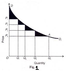
OQ1 unit at OP1price, Q1Q2 unit at OPprice, Q2Q3 unit at OP3 price and Q3Q4 unit at OP4 price. The total revenue (or price) obtained by him would be OQ4 AD. This area is the maximum expenditure that the consumers are willing to incur to buy all four units of the product under the first-degree discriminator’s all-or-nothing offer. But with no price discrimination under simple monopoly, the monopolist would sell all four units at the uniform price OP4 and thus obtain the total revenue of OQ4AP4.

This area represents the total expenditure that consumers would actually pay for the four units. Thus the difference between what Quantity the consumers were willing to pay (OQ4 AD) under Fig. 1 the take-it-or-leave-it offer of the first degree discrimi­nator and what they actually pay (OQ4AP4) to the simple monopolist, is consumers’ surplus. This is equal to the area of the triangle DAP4.

Thus under the first-degree price discrimination, the entire consumers’ surplus is pocketed by the monopolist when he charges a separate price for each unit of the product. Price discrimination of the first degree is rare and is to be found in such rare products as diamonds, jewels, precious stones, etc. But a monopolist must have full knowledge of the demand curve faced by him and he should know the maximum price that the consumers are willing to pay for each unit of the product he wants to sell.

Discrimination of the Second Degree (2nd) or Multi-part Pricing

In discrimination of the second degree, the monopolist divides the consumers in different slabs or groups or blocks and charges different prices for different slabs of the same product. Since the earlier units of the product have more utility for the consumers than the later ones, the monopolist charges a higher price for the former units and reduces the price for the later units in the respective slabs.

Such discrimination is only possible if the demand of each consumer below a certain maximum price is perfectly inelastic. Electric supply companies in developed countries practice discrimination of the second degree when they charge a high rate for the first slab of kilowatts of electricity consumed. As more electricity is used, the rate falls with subsequent slabs.

Figure 2 illustrates the second degree discrimination, where DD1is the demand curve for electric­ity on the part of domestic consumers in a town. CP3 represents the cost of generating electricity, so that the electricity company charges M1P1 rate per kw. up to OM1 units. For consuming the next M1 to М2 units, the rate is lowered to M2P2. The lowest rate charged is M3P3 for M2 to M3 units. M3P3 is, however, the lowest rate which will be charged even if a con­sumer consumes more than M3 units of electricity.

If the electricity company were to charge only one rate throughout, say M3P3the total revenue would not be maximized. It would be OCP3 M3But by charg­ing different rates for different unit slabs, it gets the total revenue equal to OM3 x P1M1 + OM2 x P2M2 + OM3x P3M3 Thus the second degree discriminator would take away a part of consumers’ surplus covered by the rectangles ABEP1and BCFP2 .The shaded area in three triangles DAP1 Р1ЕР2, and P2FP3 still remains with consumers as their surplus.

The second degree price discrimination is practised by telephone companies, railways, companies supplying water, electricity and gas in developed countries where these services are available in plenty. But it is not found in developing countries like India where such services are scarce.

The differences between the first and second degree price discrimination may be noted. In the first degree discrimination, the monopolist charges a different price for each different unit of the prod­uct. But in second degree discrimination, a number of units in one slab (or group or block) are sold at the lowest price and as the slabs increase, the prices charged by the monopolist are lowered. In the case of the former the monopolist takes away the whole of consumers’ surplus. But in the latter case, the monopolist takes away only a portion of the consumers’ surplus and the other portion is left with the buyer.

Conditions under which Price Discrimination is Possible

Price discrimination is possible under following conditions:

  1. Nature of Commodity

In the first place it is said that price discrimination is possible when the nature of the commodity or service is such that there is no possibility of transference from one market to the other.

That is, the goods sold in the cheaper market cannot be resold in the dearer market; otherwise the monopolist’s purpose will be defeated.

  1. Distance of Two Markets

Price discrimination is possible when the two markets or markets are separated by large distance or tariff barriers, so that it is not possible to transfer goods from a cheaper market to dearer markets. For instance, a monopolist may sell the same product at a higher price in Bombay and lower price in Meerut.

  1. Ignorance of the Consumers

Price discrimination is possible when the consumers are ignorant about price discrimination, they are not aware that in one part of the market prices are lower than in the other part. Thus, he purchases in dearer market, than in cheaper market since he is ignorant of the prices that are prevailing in different markets.

  1. Government Regulation

Price discrimination occurs when the government rules and regulations permit. For instance, according to rules, electricity rates are fixed at higher level for industrial purposes and lower for domestic uses. Similarly, railways charge by law higher fares from first class passengers than from the second class passengers. Hence, price discrimination is possible because of legal sanction.

  1. Geographical Discrimination

Price discrimination may be possible on account of geographical situations. The monopolist may discriminate between home and foreign buyers by selling at lower price in the foreign market than in the domestic market. Geographical discrimination is possible because no unit of the commodity sold in one market can be transferred to another.

  1. Difference in Elasticity of Demand

A commodity may have different elasticity of demand in different markets. Thus, the market of a commodity can be separated on the basis of its elasticity of demand.

Hence, a monopolist can charge different prices in different markets classified on the basis of elasticity of demand, low price is charged where demand is more elastic and high price in the market with the less elastic demand or inelastic demand.

  1. Artificial Difference between Goods

A monopolist may create artificial differences by presenting the same commodity under different names and labels, one for the rich and snobbish buyers and the other for the ordinary customers. For instance, a biscuit manufacturer may wrap small quantity of the biscuits, give it separate name and charge a higher price. Thus, he may charge different price for substantially the same product. He may charge Rs. 2/- for 100 gram wrapped biscuits and Rs. 1.50 for unwrapped biscuits.

Price Discrimination under Monopoly and Necessary Condition

Price discrimination is a selling strategy that charges customers different prices for the same product or service, based on what the seller thinks they can get the customer to agree to. In pure price discrimination, the seller charges each customer the maximum price he or she will pay. In more common forms of price discrimination, the seller places customers in groups based on certain attributes and charges each group a different price.

Price discrimination is most valuable when the profit that is earned as a result of separating the markets is greater than the profit that is earned as a result of keeping the markets combined. Whether price discrimination works and for how long the various groups are willing to pay different prices for the same product depends on the relative elasticities of demand in the sub-markets. Consumers in a relatively inelastic submarket pay a higher price, while those in a relatively elastic sub-market pay a lower price.

[Important: Price discrimination charges customers different prices for the same products based on a bias toward groups of people with certain characteristics—such as educators versus the general public, domestic users versus international users, or adults versus senior citizens.]

With price discrimination, the company looking to make the sales identifies different market segments, such as domestic and industrial users, with different price elasticities. Markets must be kept separate by time, physical distance, and nature of use.

For example, Microsoft Office Schools edition is available for a lower price to educational institutions than to other users. The markets cannot overlap so that consumers who purchase at a lower price in the elastic sub-market could resell at a higher price in the inelastic sub-market. The company must also have monopoly power to make price discrimination more effective.

Price Discrimination under Monopoly

In monopoly, there is a single seller of a product called monopolist. The monopolist has control over pricing, demand, and supply decisions, thus, sets prices in a way, so that maximum profit can be earned.

The monopolist often charges different prices from different consumers for the same product. This practice of charging different prices for identical product is called price discrimination.

According to Robinson, “Price discrimination is charging different prices for the same product or same price for the differentiated product.”

According to Stigler, “Price discrimination is the sale of various products at prices which are not proportional to their marginal costs.

In the words of Dooley, “Discriminatory monopoly means charging different rates from different customers for the same good or service.”

According to J.S. Bains, “Price discrimination refers strictly to the practice by a seller to charging different prices from different buyers for the same good.”

Necessary Conditions for Price Discrimination

Price discrimination implies charging different prices for identical goods.

It is possible under the following conditions:

(i) Existence of Monopoly

Implies that a supplier can discriminate prices only when there is monopoly. The degree of the price discrimination depends upon the degree of monopoly in the market.

(ii) Separate Market

Implies that there must be two or more markets that can be easily separated for discriminating prices. The buyer of one market cannot move to another market and goods sold in one market cannot be resold in another market.

(iii) No Contact between Buyers

Refers to one of the most important conditions for price discrimination. A supplier can discriminate prices if there is no contact between buyers of different markets. If buyers in one market come to know that prices charged in another market are lower, they will prefer to buy it in other market and sell in own market. The monopolists should be able to separate markets and avoid reselling in these markets.

(iv) Different Elasticity of Demand

Implies that the elasticity of demand in the markets should differ from each other. In markets with high elasticity of demand, low price will be charged, whereas in markets with low elasticity of demand, high prices will be charged. Price discrimination fails in case of markets having same elasticity- of demand.

Types of Price Discrimination

Price discrimination is a common pricing strategy’ used by a monopolist having discretionary pricing power. This strategy is practiced by the monopolist to gain market advantage or to capture market position.

  1. Personal

Refers to price discrimination when different prices are charged from different individuals. The different prices are charged according to the level of income of consumers as well as their willingness to purchase a product. For example, a doctor charges different fees from poor and rich patients.

  1. Geographical

Refers to price discrimination when the monopolist charges different prices at different places for the same product. This type of discrimination is also called dumping.

  1. On the basis of use

Occurs when different prices are charged according to the use of a product. For instance, an electricity supply board charges lower rates for domestic consumption of electricity and higher rates for commercial consumption.

Conditions for Price Discrimination

Price discrimination is possible under the following conditions:

  • The seller must have some control over the supply of his product. Such monopoly power is necessary to discriminate the price.
  • The seller should be able to divide the market into at least two sub-markets (or more).
  • The price-elasticity of the product must be different in different markets. Therefore, the monopolist can set a high price for those buyers whose price-elasticity of demand for the product is less than 1. In simple words, even if the seller increases the price, such buyers do not reduce the purchase volume.
  • Buyers from the low-priced market should not be able to sell the product to buyers from the high-priced market.

Hence, we can conclude that a monopolist who employs price discrimination, charges a higher price from the market with inelastic demand. On the other hand, the market which is more responsive is charged less.

Difference between price discrimination and product differentiation

  • Charging different prices for similar goods is not pure price discrimination
  • Product differentiation gives a supplier greater control over price and the potential to charge consumers a premium price arising from differences in the quality or performance of a product

Pricing Theory: Pricing Under Different Market Conditions (Perfect Competition, Imperfect Competition and Monopoly)

The theory of price is an economic theory whereby the price for any specific good or service is based on the relationship between supply and demand. The theory of price posits that the point at which the benefit gained from those who demand the entity meets the seller’s marginal costs is the most optimal market price for the good or service.

The theory of price, or price theory, is a microeconomic principle that uses the concept of supply and demand to determine the appropriate price point for a good or service. The goal is to achieve the equilibrium where the quantity of the goods or services provided match the demand of the corresponding market and its ability to acquire the good or service. The concept allows for price adjustments as market conditions change.

For example, suppose that market forces determine that a widget costs $5. A widget buyer is, therefore, willing to forgo the utility in $5 to possess the widget, and the widget seller perceives that $5 is a fair price for the widget. This simple theory of determining prices is one of the core principles underlying economic theory.

Pricing under different market conditions

  1. Perfect Competition

A perfectly competitive market is one in which the number of buyers and sellers is very large, all engaged in buying and selling a homogeneous product without any artificial restrictions and possessing perfect knowledge of market at a time. In the words of A. Koutsoyiannis, “Perfect competition is a market structure characterised by a complete absence of rivalry among the individual firms.” According to R.G. Lipsey, “Perfect competition is a market structure in which all firms in an industry are price- takers and in which there is freedom of entry into, and exit from, industry.”

Characteristics of Perfect Competition

The following are the conditions for the existence of perfect competition:

(a) Large Number of Buyers and Sellers

The first condition is that the number of buyers and sellers must be so large that none of them individually is in a position to influence the price and output of the industry as a whole. The demand of individual buyer relative to the total demand is so small that he cannot influence the price of the product by his individual action.

Similarly, the supply of an individual seller is so small a fraction of the total output that he cannot influence the price of the product by his action alone. In other words, the individual seller is unable to influence the price of the product by increasing or decreasing its supply.

Rather, he adjusts his supply to the price of the product. He is “output adjuster”. Thus no buyer or seller can alter the price by his individual action. He has to accept the price for the product as fixed for the whole industry. He is a “price taker”.

(b) Freedom of Entry or Exit of Firms

The next condition is that the firms should be free to enter or leave the industry. It implies that whenever the industry is earning excess profits, attracted by these profits some new firms enter the industry. In case of loss being sustained by the industry, some firms leave it.

(c) Homogeneous Product

Each firm produces and sells a homogeneous product so that no buyer has any preference for the product of any individual seller over others. This is only possible if units of the same product produced by different sellers are perfect substitutes. In other words, the cross elasticity of the products of sellers is infinite.

No seller has an independent price policy. Commodi­ties like salt, wheat, cotton and coal are homogeneous in nature. He cannot raise the price of his product. If he does so, his customers would leave him and buy the product from other sellers at the ruling lower price.

The above two conditions between themselves make the average revenue curve of the individual seller or firm perfectly elastic, horizontal to the X-axis. It means that a firm can sell more or less at the ruling market price but cannot influence the price as the product is homogeneous and the number of sellers very large.

(d) Absence of Artificial Restrictions

The next condition is that there is complete openness in buying and selling of goods. Sellers are free to sell their goods to any buyers and the buyers are free to buy from any sellers. In other words, there is no discrimination on the part of buyers or sellers.

Moreover, prices are liable to change freely in response to demand-supply conditions. There are no efforts on the part of the producers, the government and other agencies to control the supply, demand or price of the products. The movement of prices is unfettered.

(e) Profit Maximization Goal

Every firm has only one goal of maximizing its profits.

(f) Perfect Mobility of Goods and Factors

Another requirement of perfect competition is the perfect mobility of goods and factors between industries. Goods are free to move to those places where they can fetch the highest price. Factors can also move from a low-paid to a high-paid industry.

(g) Perfect Knowledge of Market Conditions

This condition implies a close contact between buyers and sellers. Buyers and sellers possess complete knowledge about the prices at which goods are being bought and sold, and of the prices at which others are prepared to buy and sell. They have also perfect knowledge of the place where the transactions are being carried on. Such perfect knowledge of market conditions forces the sellers to sell their product at the prevailing market price and the buyers to buy at that price.

(h) Absence of Transport Costs

Another condition is that there are no transport costs in carry­ing of product from one place to another. This condition is essential for the existence of perfect compe­tition which requires that a commodity must have the same price everywhere at any time. If transport costs are added to the price of the product, even a homogeneous commodity will have different prices depending upon transport costs from the place of supply.

(i) Absence of Selling Costs

Under perfect competition, the costs of advertising, sales-promotion, etc. do not arise because all firms produce a homogeneous product.

Perfect Competition vs Pure Competition

Perfect competition is often distinguished from pure competition, but they differ only in degree. The first five conditions relate to pure competition while the remaining four conditions are also required for the existence of perfect competition. According to Chamberlin, pure competition means, competi­tion unalloyed with monopoly elements,” whereas perfect competition involves perfection in many other respects than in the absence of monopoly.” The practical importance of perfect competition is not much in the present times for few markets are perfectly competitive except those for staple food products and raw materials. That is why, Chamberlin says that perfect competition is a rare phenomenon.”

Though the real world does not fulfill the conditions of perfect competition, yet perfect competi­tion is studied for the simple reason that it helps us in understanding the working of an economy, where competitive behaviour leads to the best allocation of resources and the most efficient organization of production. A hypothetical model of a perfectly competitive industry provides the basis for appraising the actual working of economic institutions and organizations in any economy.

  1. Imperfect Competition

Imperfect competition exists whenever a market, hypothetical or real, violates the abstract tenets of neoclassical pure or perfect competition. The contemporary theory of imperfect versus perfect competition stems from the Cambridge tradition of post-classical economic thought.

Characteristics of Imperfect competition

(i) Large number of Sellers and Buyers

There are large numbers of sellers in the market. All these firms are small sized. It means that each firm produces or sells such an insignificant portion of the total output or sale that it cannot influence the market price by its individual action. No firm can affect the sales of any other firm either by increasing or reducing its output; so there is no reaction from other firms. Every firm acts independently without bothering about the reactions of its rivals. There are a large number of buyers and none of them can affect price by his individual action.

(ii) Product Differentiation

Another important characteristic is product differentiation. The product of each seller may be similar to, but not identical with the product of other sellers in the industry. For example, a packet of Verka butter may be similar in kind to another packet of Vita butter, but because of the idea that there are differences, real or imaginary, in the quality of these two products, each buyer may have a definite preference for the one rather than for the other. As a result, each firm will have a group of buyers who prefer, for one reason or another, the product of that particular firm.

(iii) Selling Costs

Another important characteristic of the monopolistic competition is existence of selling costs. Since there is product differentiation and products are close substitutes, selling costs are important to persuade buyers to change their preferences, so as to raise their demand for a given article. Under monopolistic competition, advertisement is not only persuasive but also informatory because a large number of firms are operating in the market and buyer’s knowledge about the market is not perfect.

(iv) Free Entry and exit of Firms

Firms under monopolistic competition are free to join and leave the industry at any time they like to. The implication of this characteristic is that by entering freely into the market, the firms can produce close substitutes and increase the supply of commodity in the market. Similarly, the firm commands such a meager amount of resources that in the event of losses, they may easily quit the market.

(v) Price makers

In the monopolistic competitive market, each firm is a price-maker as it can determine the price of its own brand of the product.

(vi) Blend of Competition and Monopoly

In this market, each firm has a monopoly power over its product as it would not lose all customers if it raises the price as its product is not perfect substitute of other brands. At the same time, there is an element of competition because the consumers treat the different firms’ products as close substitutes. Hence, if a firm raises the price of its brand, it would lose some customers to other brands.

  1. Monopoly Market

Monopoly is a market situation in which there is only one seller of a product with barriers to entry of others. The product has no close substitutes. The cross elasticity of demand with every other product is very low. This means that no other firms produce a similar product. According to D. Salvatore, “Monopoly is the form of market organization in which there is a single firm selling a commodity for which there are no close substitutes.” Thus the monopoly firm is itself an industry and the monopolist faces the industry demand curve.

The demand curve for his product is, therefore, relatively stable and slopes downward to the right, given the tastes, and incomes of his customers. It means that more of the product can be sold at a lower price than at a higher price. He is a price-maker who can set the price to his maximum advantage.

However, it does not mean that he can set both price and output. He can do either of the two things. His price is determined by his demand curve, once he selects his output level. Or, once he sets the price for his product, his output is determined by what consumers will take at that price. In any situation, the ultimate aim of the monopolist is to have maximum profits.

Characteristics of Monopoly

The main features of monopoly are as follows:

  • Under monopoly, there is one producer or seller of a particular product and there is no differ­ence between a firm and an industry. Under monopoly a firm itself is an industry.
  • A monopoly may be individual proprietorship or partnership or joint stock company or a co­operative society or a government company.
  • A monopolist has full control on the supply of a product. Hence, the elasticity of demand for a monopolist’s product is zero.
  • There is no close substitute of a monopolist’s product in the market. Hence, under monopoly, the cross elasticity of demand for a monopoly product with some other good is very low.
  • There are restrictions on the entry of other firms in the area of monopoly product.
  • A monopolist can influence the price of a product. He is a price-maker, not a price-taker.
  • Pure monopoly is not found in the real world.
  • Monopolist cannot determine both the price and quantity of a product simultaneously.
  • Monopolist’s demand curve slopes downwards to the right. That is why, a monopolist can increase his sales only by decreasing the price of his product and thereby maximize his profit. The marginal revenue curve of a monopolist is below the average revenue curve and it falls faster than the average revenue curve. This is because a monopolist has to cut down the price of his product to sell an additional unit.

Market Structure, Meaning, Elements, Factors influencing Market Structure

Market structure refers to the organizational and competitive characteristics of a market that influence the behavior and performance of the firms operating within it. It defines how businesses interact with each other, how prices are determined, and how easily new firms can enter or exit the market.

Elements or Determinants of Market Structure:

  • Number of Buyers and Sellers

The number of buyers and sellers in a market determines the degree of competition and price influence. In a perfectly competitive market, numerous sellers exist, none of which can individually influence price. In contrast, a monopoly has a single seller with complete price control. An oligopoly features a few dominant firms, often engaging in strategic pricing and product decisions. The greater the number of sellers, the more competitive the market becomes, leading to better choices and prices for consumers. On the buyer side, the presence of many buyers ensures demand diversity and minimizes buyer influence. If a few large buyers dominate (monopsony), they may exert significant control over prices and terms. Thus, the balance of buyers and sellers shapes the market’s competitive nature.

  • Nature of the Product

The type of product offered—whether homogeneous or differentiated—significantly influences market structure. In perfect competition, products are identical (e.g., wheat, salt), leaving firms with no control over pricing. In monopolistic competition, products are similar but differentiated by branding, quality, or features (e.g., clothing brands), allowing some pricing power. In oligopoly, products may be either homogeneous (e.g., cement) or differentiated (e.g., automobiles), and product features become strategic tools for competition. In a monopoly, the firm offers a unique product with no close substitutes, granting it full pricing authority. Product nature affects customer loyalty, elasticity of demand, and marketing strategies. The greater the product differentiation, the more power a firm has to set prices and influence consumer choices.

  • Degree of Price Control

Price control refers to the extent to which a firm can influence the price of its product. In perfect competition, firms are price takers—they accept market-determined prices due to intense competition and identical products. In monopolistic competition, firms have limited pricing power due to brand loyalty and differentiation. In oligopolies, firms have considerable price control, but often follow price leadership or engage in collusive pricing to avoid price wars. A monopolist, on the other hand, is a price maker, setting prices to maximize profits, although constrained by consumer demand and potential regulation. The degree of price control depends on factors like product uniqueness, market entry barriers, and consumer sensitivity. Understanding price control helps assess market power and the potential for consumer exploitation or competitive pricing.

  • Entry and Exit Barriers

Ease of market entry and exit is a key element of market structure, affecting the level of competition and innovation. In perfect competition, there are no barriers, allowing new firms to enter freely and keep profits in check. In monopolistic competition, entry is relatively easy, though branding may pose minor challenges. In oligopoly, high entry barriers such as heavy capital investment, economies of scale, and control over distribution prevent new competitors from entering. In a monopoly, barriers are the highest, often due to patents, government licenses, or ownership of key resources. These barriers protect existing firms from competition, allowing them to maintain profits and influence. Lower entry and exit barriers promote market dynamism, while higher barriers can lead to reduced competition, higher prices, and consumer disadvantage.

Factors influencing Market Structure:

  • Number of Firms in the Market

The number of firms determines the level of competition in a market. A large number of firms typically results in a competitive structure like perfect or monopolistic competition, where no single firm dominates. Fewer firms may lead to oligopoly or monopoly, where market power is concentrated. The higher the number of firms, the less control each has over pricing and supply. This factor directly affects how freely new businesses can enter the market, influence prices, and affect consumer choices, shaping the overall structure and nature of business rivalry.

  • Nature of the Product

The similarity or differentiation of products significantly impacts market structure. Homogeneous products, such as grains or steel, lead to perfect competition, where firms compete solely on price. Differentiated products, like branded clothing or electronics, result in monopolistic competition or oligopoly, where firms gain some price control through branding and features. A unique product with no substitutes, as seen in a monopoly, gives complete pricing power to the firm. The more distinct the product, the higher the potential for firms to establish loyal customer bases and exercise market influence.

  • Control Over Prices

The degree of control firms have over pricing determines their influence in the market. In perfect competition, firms are price takers—they cannot alter prices due to intense rivalry. In monopoly, a firm is a price maker, controlling prices due to a lack of substitutes. Oligopolistic firms have considerable price-setting power but often avoid price wars through collusion or tacit agreements. Price control is shaped by product uniqueness, brand value, and the availability of alternatives. More price control indicates less competition and a more concentrated market structure.

  • Barriers to Entry and Exit

Barriers affect how easily new firms can enter or leave a market. Low barriers promote competition, as seen in perfect and monopolistic competition. High barriers, like legal restrictions, high startup costs, and access to technology, protect established firms in oligopolies and monopolies, reducing competition. These barriers determine market dynamics, profitability, and innovation levels. The ease or difficulty of entering the market shapes the competitive intensity, and hence, the overall market structure. Exit barriers, such as long-term contracts or sunk costs, also influence firms’ decisions and market fluidity.

  • Economies of Scale

When firms grow large enough to lower average costs through mass production, they experience economies of scale. This factor influences market structure by favoring oligopolies and monopolies, where large firms dominate due to cost advantages. Smaller firms find it difficult to compete, leading to a concentrated market. The presence of economies of scale raises entry barriers, discouraging new entrants and reducing competition. Industries like telecom, aviation, and energy often display this trait. This factor strengthens the position of existing firms and shapes the strategic behavior in the industry.

  • Level of Innovation and Technology

High levels of innovation and advanced technology can significantly affect market structure. In tech-driven industries, early adopters often gain a temporary monopoly due to patents, proprietary processes, or first-mover advantages. Rapid innovation can reduce entry barriers if technology is widely accessible, but may also create new barriers when it involves complex, capital-intensive processes. Innovation leads to product differentiation, changing competitive dynamics and often shifting markets from monopolistic to oligopolistic forms. It influences firm growth, pricing strategies, and the overall shape of market competition.

  • Government Policies and Regulations

Government intervention through licensing, tariffs, price controls, and antitrust laws significantly influences market structure. Policies that encourage free trade and deregulation promote competition, while those granting monopoly rights or subsidies can limit it. Regulatory frameworks may either lower or raise entry barriers, depending on their objectives. For instance, strict patent laws can create monopolies, while competition laws may break up large firms. These rules impact pricing, market access, and competitive fairness, playing a crucial role in shaping the structure and efficiency of different markets.

The features of market structures are shown in Table 1.

Important features of market structure:

  • Number and Size of Buyers and Sellers

The number and relative size of buyers and sellers directly influence the nature of competition in a market. In perfect competition, there are many small buyers and sellers, so no single entity can influence the price. In contrast, monopoly features one large seller dominating the entire market. Oligopoly has few large sellers, while monopolistic competition has many sellers offering differentiated products. The balance of power between buyers and sellers determines price-setting behavior, market entry, and overall market dynamics.

  • Nature of the Product

Products can be homogeneous (identical) or differentiated. Homogeneous goods (e.g., wheat, sugar) are typical of perfect competition, where consumers have no preference between suppliers. Differentiated products (e.g., smartphones, clothing) are associated with monopolistic competition or oligopoly, where branding and features give firms some pricing power. In monopoly, the product is unique with no close substitutes. The product’s nature shapes consumer choice, pricing strategy, and firm competitiveness, making it a key feature in defining the structure of a market.

  • Degree of Price Control

Price control refers to how much influence firms have over the price of their products. In perfect competition, firms are price takers, accepting market-determined prices. In contrast, monopolies are price makers, having full control due to lack of substitutes. Oligopolies have partial control and often avoid price wars through mutual understanding. Monopolistic competitors can influence prices slightly due to product differentiation. The ability to control prices affects profitability, strategic planning, and the level of consumer surplus in different market structures.

  • Entry and Exit Conditions

The ease with which firms can enter or exit the market impacts the level of competition. Free entry and exit, seen in perfect and monopolistic competition, keeps profits normal in the long run. High entry barriers in monopoly and oligopoly markets, such as large capital requirements, patents, and government regulations, protect existing firms from new competitors. These conditions influence firm behavior, investment decisions, and the long-term structure of the industry. Exit barriers also matter, including sunk costs and contractual obligations.

  • Flow of Information

Market transparency, or the availability of information, significantly impacts decision-making. In perfect competition, information is perfect and freely available to all participants, ensuring rational decisions and uniform prices. In monopoly, oligopoly, or monopolistic competition, information may be asymmetric—some firms have better access to market data, customer preferences, or production techniques. Information asymmetry leads to inefficiencies, mispricing, and poor resource allocation. The better the information flow, the more efficient and competitive the market structure becomes.

  • Interdependence Among Firms

In oligopoly, firms are highly interdependent; the actions of one firm significantly impact others. For example, a price cut by one may trigger retaliatory pricing. In monopoly and perfect competition, interdependence is minimal—monopolies face no rivals, and perfect competitors are too small to affect market outcomes. Monopolistic competition lies in between, with firms competing based on product features. This interdependence influences strategic behavior, including pricing, advertising, and innovation, and it makes game theory and collusion relevant in oligopolistic settings.

  • Government Regulation and Legal Framework

Government rules and policies shape the nature and behavior of market structures. Antitrust laws, price controls, trade regulations, and licensing influence how freely firms can operate, compete, or dominate. Monopolies may be state-sanctioned, while competitive markets are supported by policies promoting transparency and consumer rights. Legal restrictions may also create barriers to entry, affecting the long-term dynamics of the industry. In regulated markets, government action balances business interests with consumer welfare, playing a crucial role in defining market behavior and structure.

  • Profit Margins and Cost Efficiency

The structure of a market significantly impacts potential profit margins and cost structures. Perfect competition leads to minimal profit margins due to intense competition and price pressure. In contrast, monopolies enjoy higher profit margins due to price-setting power and absence of competition. Oligopolistic firms also enjoy significant profits through collusion or differentiated services. Monopolistic competitors rely on brand value to maintain margins. Additionally, cost efficiency varies—larger firms may benefit from economies of scale, leading to lower average costs and higher profitability in certain structures.

Types of market structure:

1. Perfect Competition

Perfect competition is an idealized market structure where a large number of small firms sell identical products. No single firm can influence the price, making them price takers. The product is homogeneous, and all buyers and sellers have perfect knowledge. Entry and exit are completely free, and there is no government intervention. Examples include agricultural markets like wheat or rice, where products are uniform and pricing is dictated by market forces. Long-run profits tend toward normal, and efficiency is maximized.

2. Monopoly

A monopoly exists when a single firm dominates the entire market with no close substitutes for its product. The firm is a price maker, meaning it has full control over the price. High entry barriers such as patents, licenses, large capital requirements, or government protection prevent other firms from entering. Consumers have limited choices, and the monopolist maximizes profit by producing where marginal cost equals marginal revenue. Examples include utilities like electricity and water supply in many regions.

3. Monopolistic Competition

This structure features many sellers offering similar but differentiated products. Firms have some price-setting power due to brand identity, quality, packaging, or advertising. Entry and exit are relatively easy, and information is fairly well distributed among buyers and sellers. This market is common in retail sectors like clothing, restaurants, or consumer electronics, where consumers perceive differences in brands even if the underlying product is similar. Firms compete on both price and non-price factors like style, location, and service.

4. Oligopoly

In an oligopoly, a few large firms dominate the market. Products may be homogeneous (e.g., steel, cement) or differentiated (e.g., cars, smartphones). Firms are interdependent and often respond to each other’s actions—especially regarding pricing and output. Barriers to entry are high, which keeps competition limited. Pricing may be rigid due to fear of price wars. Strategic planning and collusion (formal or informal) are common. Real-world examples include the airline industry, telecom sector, and automobile manufacturing.

Break Even Point: Meaning, Features and Significance

Break-even point represents that volume of production where total costs equal to total sales revenue resulting into a no-profit no-loss situation.

In simple words, the break-even point can be defined as a point where total costs (expenses) and total sales (revenue) are equal. Break-even point can be described as a point where there is no net profit or loss. The firm just “breaks even.” Any company which wants to make abnormal profit, desires to have a break-even point. Graphically, it is the point where the total cost and the total revenue curves meet.

Calculation (formula)

Break-even point is the number of units (N) produced which make zero profit.

Revenue – Total costs = 0

Total costs = Variable costs * N + Fixed costs

Revenue = Price per unit * N

Price per unit * N – (Variable costs * N + Fixed costs) = 0

So, break-even point (N) is equal

N = Fixed costs / (Price per unit – Variable costs)

About Break-even point

The origins of break-even point can be found in the economic concepts of “the point of indifference.” Calculating the break-even point of a company has proved to be a simple but quantitative tool for the managers. The break-even analysis, in its simplest form, facilitates an insight into the fact about revenue from a product or service incorporates the ability to cover the relevant production cost of that particular product or service or not. Moreover, the break-even point is also helpful to managers as the provided info can be used in making important decisions in business, for example preparing competitive bids, setting prices, and applying for loans.

Adding more to the point, break-even analysis is a simple tool defining the lowest quantity of sales which will include both variable and fixed costs. Moreover, such analysis facilitates the managers with a quantity which can be used to evaluate the future demand. If, in case, the break-even point lies above the estimated demand, reflecting a loss on the product, the manager can use this info for taking various decisions. He might choose to discontinue the product, or improve the advertising strategies, or even re-price the product to increase demand.

Another important usage of the break-even point is that it is helpful in recognizing the relevance of fixed and variable cost. The fixed cost is less with a more flexible personnel and equipment thereby resulting in a lower break-even point. The importance of break-even point, therefore, cannot be overstated for a sound business and decision making.

However, the applicability of break-even analysis is affected by numerous assumptions. A violation of these assumptions might result in erroneous conclusions.

Features of Break Even Point

(i) It helps in the determination of selling price which will give the desired profits.

(ii) It helps in the fixation of sales volume to cover a given return on capital employed.

(iii) It helps in forecasting costs and profit as a result of change in volume.

(iv) It gives suggestions for shift in sales mix.

(v) It helps in making inter-firm comparison of profitability.

(vi) It helps in determination of costs and revenue at various levels of output.

(vii) It is an aid in management decision-making (e.g., make or buy, introducing a product etc.), forecasting, long-term planning and maintaining profitability.

(viii) It reveals business strength and profit earning capacity of a concern without much difficulty and effort.

Significance of Break Even Point

(i) All costs can be separated into fixed and variable components

(ii) Fixed costs will remain constant at all volumes of output

(iii) Variable costs will fluctuate in direct proportion to volume of output

(iv) Selling price will remain constant

(v) Product-mix will remain unchanged

(vi) The number of units of sales will coincide with the units produced so that there is no opening or closing stock

(vii) Productivity per worker will remain unchanged

(viii) There will be no change in the general price level

Limitations of Break-Even Analysis

  1. Break-even analysis is based on the assumption that all costs and expenses can be clearly separated into fixed and variable components. In practice, however, it may not be possible to achieve a clear-cut division of costs into fixed and variable types.
  2. It assumes that fixed costs remain constant at all levels of activity. It should be noted that fixed costs tend to vary beyond a certain level of activity.
  3. It assumes that variable costs vary proportionately with the volume of output. In practice, they move, no doubt, in sympathy with volume of output, but not necessarily in direct proportions..
  4. The assumption that selling price remains unchanged gives a straight revenue line which may not be true. Selling price of a product depends upon certain factors like market demand and supply, competition etc., so it, too, hardly remains constant.
  5. The assumption that only one product is produced or that product mix will remain unchanged is difficult to find in practice.
  6. Apportionment of fixed cost over a variety of products poses a problem.
  7. It assumes that the business conditions may not change which is not true.
  8. It assumes that production and sales quantities are equal and there will be no change in opening and closing stock of finished product, these do not hold good in practice.
  9. The break-even analysis does not take into consideration the amount of capital employed in the business. In fact, capital employed is an important determinant of the profitability of a concern.

Cost: Output Relationship in Short and Long Run

Cost Output Relationship in Short Run

Time element plays an important role in price determination of a firm. During short period two types of factors are employed. One is fixed factor while others are variable factors of production. Fixed factor of production remains constant while with the increase in production, we can change variable inputs only because time is short in which all the factors cannot be varied.

Raw material, semi-finished material, unskilled labour, energy, etc., are variable inputs which can be changed during short run. Machines, capital, infrastructure, salaries of managers and technical experts are included in fixed inputs. During short period an individual firm can change variable factors of production according to requirements of production while fixed factors of production cannot be changed.

Cost-Output Relationship in the Short Run:

(i) Average Fixed Cost Output

The greater the output, the lesser the fixed cost per unit, i.e., the average fixed cost. The reason is that total fixed costs remain the same and do not change with a change in output.

The relationship between output and fixed cost is a universal one for all types of business.

Thus, average fixed cost falls continuously as output rises. The reason why total fixed costs remain the same and the average fixed cost falls is that certain factors are indivisible. Indivisibility means that if a smaller output is to be produced, the factor cannot be used in a smaller quantity. It is to be used as a whole.

(ii) Average Variable Cost and Output

The average variable costs will first fall and then rise as more and more units are produced in a given plant. This is so because as we add more units of variable factors in a fixed plant, the efficiency of the inputs first increases and then decreases. In fact, the variable factors tend to produce somewhat more efficiently near a firm’s optimum output than at very low levels of output.

But once the optimum capacity is reached, any further increase in output will undoubtedly increase average variable cost quite sharply. Greater output can be obtained but at much greater average variable cost. For example, if more and more workers are appointed. It may ultimately lead to overcrowding and bad organization. Moreover, workers may have to be paid higher wages for overtime work.

(iii) Average Total Cost and Output

Average total costs, more commonly known as average costs, will decline first and then rise upward. The significant point to note here is that the turning point in the case of average cost comes a little later in the case of average variable cost.

Average cost consists of average fixed cost plus average variable cost. As we have seen, average fixed cost continues to fall with an increase in output while average variable cost first declines and then rises. So long as average variable cost declines the average total cost will also decline. But after a point, the average variable cost will rise. Here, if the rise in variable cost is less than the drop in fixed cost, the average total cost will still continue to decline.

It is only when the rise in average variable cost is more than the drop in average fixed cost that the average total cost will show a rise. Thus, there will be a stage where the average variable cost may have started rising yet the average total cost is still declining because the rise in average variable cost is less than the drop in average fixed cost. The net effect being a decline in average cost.

The least cost-output level is the level where the average total cost is the minimum and not the average variable cost. In fact, at the least cost-output level, the average variable cost will be more than its minimum (average variable cost). The least cost- output level is also the optimum output level. It may not be the maximum output level. A firm may decide to produce more than the least cost-output level.

(iv) Short-Run Output Cost Curves

The cost-output relationships can also be shown through the use of graphs. It will be seen that the average fixed cost curve (AFC curve) falls as output rises from lower levels to higher levels. The shape of the average fixed cost curve, therefore, is a rectangular hyperbola.

However, the average variable cost curve (AVC curve) starts rising earlier than the ATC curve. Further, the least cost level of output corresponds to the point LT on the ATC curve and not to the point LV which lies on the AVC curve.

Another important point to be noted is that in Fig. the marginal cost curve (MC curve) intersects both the AVC curve and ATC curve at their minimum points. This is very simple to explain. If marginal cost (MC) is less than the average cost (AC), it will pull AC down. If the MC is greater than AC, it will pull AC up. If the MC is equal to AC, it will neither pull AC up nor down. Hence, MC curve tends to intersect the AC curve at its lowest point.

Similar is the position about the average variable cost curve. It will not make any difference whether MC is going up or down. LT is the lowest point of total cost and LV is the lowest point of variable cost.

The inter-relationships among AVC, ATC, and AFC can be summed up as follows:

  • If both AFC and AVC fall, ATC will also fall.
  • If AFC falls but AVC rises

(a) ATC will fall where the drop in AFC is more than the rise in AVC.

(b) ATC will not fall where the drop in AFC is equal to the rise in AVC.

(c) ATC will rise where the drop in AFC is less than the rise in AVC.

Cost Output Relationship in Long Run

The long run is a period long enough to make all costs variable including such costs as are fixed in the short run. In the short run, variations in output are possible only within the range permitted by the existing fixed plant and equipment. But in the long run, the entrepreneur has before him a number of alternatives which includes the construction of various kinds and sizes of plants.

Thus, there are no fixed costs since the firm has sufficient time to fully adapt its plant. And all costs become variable. In view of this, the long-run costs will refer to the costs of producing different levels of output by changes in the size of plant or scale of production. The long-run cost-output relationship is shown graphically by the long- run cost curve—a curve showing how costs will change when the scale of production is changed.

The concept of long-run costs can be further explained with the help of an illustration. Suppose that at a particular time, a firm operates under average total cost curve U2 and produces OM. Now it is desired to produce ON. If the firm continues under the old scale, its average cost curve will be NT. If the scale of firm is altered, the new cost curve will be U3. The average cost of producing ON will then be NA.

NA is less than NT. So the new scale is preferable to the old one and should be adopted. In the long run, the average cost of producing ON output is NA. This may be called as the long-run cost of producing ON output. It may be noted here that we shall call NA as the long-run cost only so long as the U3 scale is in the planning stage and has not actually been adopted. The moment the scale is installed, the NA cost will be the short-run cost of producing ON output.

To draw a long-run cost curve, we have to start with a number of short-run average cost curves (SAC curves), each such curve representing a particular scale or size of the plant, including the optimum scale. One can now draw the long-run cost curve which tangential to the entire family of SAC curves, that is, it touches each SAC curve at one point.

Cost Concepts Meaning and Types of Costs

According to the Chartered Institute of Management Accountants, cost is “the amount of expenditure (actual or notional) incurred on or attributable to a specified thing or activity.” Similarly, according to Anthony and Wilsch “cost is a measurement in monetary terms of the amount of resources used for some purposes.”

Cost has been defined by the Committee on Cost Terminology of the American Accounting Association as “the foregoing, in monetary terms, incurred or potentially to be incurred in the realization of the objective of management which may be manufacturing of a product or rendering of a service.”

From the above, it may be stated that cost means the total of all expenses incurred for a product or a service. Thus, cost of an article means the actual outgoings or ascertained changes incurred in its production and sale activities. In short, it is the amount of resources used up in exchange for some goods or services.

The so-called resources are expressed in terms of money or monetary units. What we stated above will not be a meaningful one until the same is used with an adjective only, i.e. when it communicates the meaning for which it is intended.

Thus, when we say Prime Cost or Works Cost or Fixed Cost etc., we want to explain a particular meaning which is essential while computing, measuring or analyzing the various aspects of cost.

Classification of Cost

Classification of costs implies the process of grouping costs according to their common characteristics. A proper classification of costs is absolutely necessary to mention the costs with cost centres. Usually, costs are classified according to their nature, viz., material, labour, over-head, among others. An identical cost figure may be classified in various ways according to the needs of the firms.

The above classification may be outlined as:

The classification of cost may be depicted as given:

  1. According to Elements

Under the circumstances, costs are classified into three broad categories Material, Labour and Overhead. Now, further subdivision may also be made for each of them. For example, Material may be subdivided into raw materials, packing materials, consumable stores etc. This classification is very useful in order to ascertain the total cost and its components. Same classification may also be made for labour and overhead.

  1. According to Functions

The total costs are divided into different segments according to the purpose of the firm. That is why costs are grouped as per the requirements of the firm in order to evaluate its functions properly. In short, the total costs include all costs starting from cost of materials to the cost of packing the product.

It takes the cost of direct material, direct labour and chargeable expenses and all indirect expenses under the head Manufacturing/Production cost.

At the same time, administration cost (i.e. relating to office and administration) and Selling and Distribution expenses (i.e. relating to sales) are to be classified separately and to be added in order to find out the total cost of the product. If these functional classifications are not made properly, true cost of the product cannot accurately be ascertained.

  1. According to Variability

Practically, costs are classified according to their behaviour relating to the change (increase or decrease) in their volume of activity.

These costs as per volume may be subdivided into:

(i) Fixed Cost

(ii) Variable Cost

(iii) Semi-variable Cost

Fixed Costs are those which do not vary with the change in output, i.e., irrespective of the quantity of output produced, it remains fixed (e.g., Salaries, Rent etc.) up to a certain limit. It is interesting to note that if more units are product, fixed cost per unit will be reduced, and, if less units are produced, obviously, fixed cost per unit will be increased.

Variable Costs, on the other hand, are those which vary proportionately with the volume of output. So the cost per unit will remain fixed irrespective of the quantity produced. That is, there is no direct effect on the cost per unit if there is a change in the volume of output (e.g. price of raw material, labour etc.,).

On the contrary, semi-variable costs are those which are partly fixed and partly variable (e.g. Repairs of building).

  1. According to Controllability

Costs may, again, be subdivided into two broad categories according to the performance done by any member of the firm.

They are:

(i) Controllable Costs; and

(ii) Uncontrollable Costs.

Controllable Costs are those costs which may be influenced by the decision taken by a specified member of the administration of the firm or, it may be stated, that the costs which at least partly depend on the management and is controllable by them, e.g. all direct costs, direct material, direct labour and chargeable expenses (components of Prime Cost) are controllable by lower management level and is done accordingly.

Uncontrollable Costs are those which are not influenced by the actions taken by any specific member of the management. For example, fixed costs, viz., rent of building, payment for salaries etc.

  1. According to Normality

Under this condition, costs are classified according to the normal needs for a given level of output for a normal level of activity produced for such output.

They are divided into:

(i) Normal Costs

(ii) Abnormal Costs

Normal Costs are those costs which are normally required for a normal production at a given level of output and which is a part of production.

Abnormal Costs, on the other hand, are those costs which are not normally required for a given level of output to be produced normally, or which is not a part of cost of production.

  1. According to Time

Costs may also be classified according to the time element in it. Accordingly, costs are classified into:

(i) Historical Costs

(ii) Predetermined Costs.

Historical Costs are those costs which are taken into consideration after they have been incurred. This is possible particularly when the production of a particular unit of output has already been made. They have only historical value and cannot assist in controlling costs.

Predetermined Costs, on the other hand, are the estimated costs. Such costs are computed in advanced on the basis of past experience and records. Needless to say here that it becomes standard cost if it is determined on scientific basis. When such standard costs are compared with the actual costs, the reasons of variance will come out which will help the management to take proper steps for reconciliation.

  1. According to Traceability

Costs can be identified with a particular product, process, department etc. They are divided into:

(i) Direct (Traceable) Costs

(ii) Indirect (Non-Traceable) Costs.

Direct/Traceable Costs are those costs which can directly be traced or allocated to a product, i.e. it includes all traceable costs, viz., all expenses relating to cost of raw materials, labour and other service utilised which can be traced easily.

Indirect/Non-Traceable Costs are those costs which cannot directly be traced or allocated to a product, i.e. it includes all non-traceable costs, e.g. salary of store-keepers, general administrative expenses, i.e. which cannot properly be allocated directly to a product.

  1. According to Planning and Control

Costs may also be classified into:

(i) Budgeted Costs

(ii) Standard Costs.

Budgeted Costs refer to the expected cost of manufacture computed on the basis of information available in advance of actual production or purchase. Practically, budgeted costs include standard costs, both are predetermined costs and their amount may coincide but their objectives are different.

Standard Costs, on the other hand, is a predetermination of what actual costs should be under projected conditions serving as a basis of cost control and, as a measure of product efficiency, when ultimately aligned actual cost. It supplies a medium by which the effectiveness of current results can be measured and the responsibility for derivations can be placed.

Standard Costs are predetermined for each element, viz., material, labour and overhead.

Standard Costs include

(i) The cost per unit is determined to make an estimated total output for the future period for:

(a) Material

(b) Labour

(c) Overhead.

(ii) The cost must depend on the past experience and experiments and specification of the technical staff.

(iii) The cost must be expressed in terms of rupees.

  1. According to Management Decisions

Under this, costs may also be classified as:

(a) Marginal Cost: Marginal Cost is the cost for producing additional unit or units by segregation of fixed costs (i.e., cost of capacity) from variable cost (i.e. cost of production) which helps to know the profitability. Moreover, we know, in order to increase the production, certain expenses (fixed) may not increase at all, only some expenses relating to materials, labour and variable expenses are increased. Thus, the total cost so increased by the production of one unit or more is the cost of marginal unit and the cost is known as marginal cost or incremental cost.

(b) Differential Cost: Differential Cost is that portion of the cost of a function attributable to and identifiable with an added feature, i.e. the change in costs as a result of change in the level of activity or method of production.

(c) Opportunity Cost: It is the prospective change in cost following the adoption of an alternative machine, process, raw materials, specification or operation. In other words, it is the maximum possible alternative earnings which might have been earned if the existing capacity had been changed to some other alternative way.

(d) Replacement Cost: It is the cost, at current prices, in a particular locality or market area, of replacing an item of property or a group of assets.

(e) Implied Cost: It is the cost used to indicate the presence of arbitrary or subjective elements of product cost having more than usual significance. It is also called notional cost, e.g., interest on capital although no interest is paid. This is particularly useful while decisions are taken regarding alternative capital investment projects.

(f) Sunk Cost: It is the past cost arising out of a decision which cannot be revised now, and associated with specialised equipment’s or other facilities not readily adaptable to present or future purposes. Such cost is often regarded as constituting a minor factor in decisions affecting the future.

Iso-Product Curves- Meaning and Features

An iso-product curve is locus of various combinations of two factors of production giving the same level of output and a producer is indifferent to each of such combinations. All the combinations of two inputs give the same quantum of output to a producer and the producer is indifferent to each such combination. He does not have any preference. These iso-product curves are also called production indifference curves. The concept of iso-product curve can be explained with the help of iso-quant schedule and diagram.

Assumptions:

The main assumptions of Iso-quant curves are as follows:

  1. Two Factors of Production:

Only two factors are used to produce a commodity.

  1. Divisible Factor:

Factors of production can be divided into small parts.

  1. Constant Technique:

Technique of production is constant or is known beforehand.

  1. Possibility of Technical Substitution:

The substitution between the two factors is technically possible. That is, production function is of ‘variable proportion’ type rather than fixed proportion.

  1. Efficient Combinations:

Under the given technique, factors of production can be used with maximum efficiency.

Iso-Quant Schedule

An iso-quant schedule shows different combinations of two factors of production (inputs) at which a producer gets equal quantum of output.

The schedule is given below:

The above schedule shows the different combinations of two inputs, namely, labour and capital and the resultant output 100 units from each combination. The units of labour are increasing and units of capital are decreasing but the quantity of output remains the same.

The schedule can be depicted in the form of a diagram given below:

In the diagram factor A and factor B are shown on OX-axis and OY-axis respectively. IP is the iso-product curve showing the different combinations (A, B, C, D and E) of the two factors of production giving the same quantity of output (100 units).

The IP curve slopes downward to the right. It explains with the increase in the units of factor-A when we are reducing the units of factor-B.

Iso-Product Curve and Indifference Curve

The shape and slope of iso-product curve and indifference curve are similar but both of them have the following differences:

(1) Iso-product curve shows the quantum of output while an indifference curve shows the level of satisfaction. Iso-product curve shows the different combinations of two factors of production (inputs) showing the same quantum of output but an indifference curve shows the different combinations of two commodities showing the same level of satisfaction.

(2) We can prepare an iso-product map by which we can express that how much less or more quantity of output is shown by each iso-product curve but an indifference curve cannot say how much more or less is the satisfaction from different combinations of two commodities a consumer is getting. Utility or satisfaction is not measurable but the quantity of output is measurable with the help of iso-product curve.

Features of Iso-Product Curves

The following are the characteristics of iso-product curves:

(1) Iso-Product Curves Slope Downward to the Right

Iso- product curves slope downward to the right because producer has limited resources with alternative uses and he is faced with the problem of choice. He cannot increase the amount of labour and capital. If he employs more of labour he has to employ less of capital in order to get the same level of output as given in the following diagram:

The diagram shows that units of labour are shown on OX- axis and units of capital on OY-axis. A combination shows OK of capital and OL of labour while at B combination OK1 of capital and OL1 of labour showing the same amount of output (100 units). But the producer has employed more of labour and less of capital and on account of it the iso-product curve slopes downward to the right.

(2) Iso-Product Curves are Convex to the Origin

As an indifference curve is convex to the origin, similarly an iso-product curve is also convex to the origin. In an iso-product curve a factor of production is substituted by another factor of production and consequently the marginal rate of technical substitution of labour for capital (MRTSLK) declines and on account of decreasing MRTSLK the iso-product curves are convex to the origin.

It is shown by the following diagram:

The table reveals that we are increasing the units of labour and reducing the units of capital. The MRTSLK shows a declining trend.

(3) Two Iso-Product Curve never Intersect Each Other

Another characteristic is that two iso-product curves do not intersect each other as different iso-product curves show different level of output.

It is shown by the following diagram:

Capital and labour are shown on OY-axis and OX-axis respectively. IP and IPX are two iso-product curves. E is the point where IP2 and IP1 intersect each other.

Before E point IP1 is higher than IP2 and after E point IP1 is higher than IP. In such a situation it is difficult to know which Iso- product curve gives higher level of output. Hence, we can say that it is indeterminate and two iso-product curves do not cut each other.

(4) Higher the Iso-Quant Curve Higher is the Level of Output

A producer gets the same level of output with different combinations of two inputs on the iso-product curve. But in case of different iso-product curves the level of output differs. Higher the iso-product curve, higher the level of output and lower the iso-product, lower will be the level of output. It can be seen from Diagram 5.

The diagram shows Iso-product map in which three Iso- product curves are showing different levels of output. IP, IP1 and IP2 are showing 500 units, 1000 units and 1500 units respectively which show increasing trends. Higher the iso-product curve higher is the level of output (IP to IP2), lower the iso-product curve lower will be the level of output (IP2 to IP). The highest iso-product curve is IP2 and the lowest iso-product curve is IP.

(5) No Isoquant can Touch Either Axis:

If an isoquant touches X-axis, it would mean that the product is being produced with the help of labour alone without using capital at all. These logical absurdities for OL units of labour alone are unable to produce anything. Similarly, OC units of capital alone cannot produce anything without the use of labour. Therefore as seen in figure 9, IQ and IQ1 cannot be isoquants.

(6) Each Isoquant is Oval-Shaped.

It means that at some point it begins to recede from each axis. This shape is a consequence of the fact that if a producer uses more of capital or more of labour or more of both than is necessary, the total product will eventually decline. The firm will produce only in those segments of the isoquants which are convex to the origin and lie between the ridge lines. This is the economic region of production. In Figure 10, oval shaped isoquants are shown.

Curves OA and OB are the ridge lines and in between them only feasible units of capital and labour can be employed to produce 100, 200, 300 and 400 units of the product. For example, OT units of labour and ST units of the capital can produce 100 units of the product, but the same output can be obtained by using the same quantity of labour T and less quantity of capital VT.

Thus only an unwise entrepreneur will produce in the dotted region of the iso-quant 100. The dotted segments of an isoquant are the waste- bearing segments. They form the uneconomic regions of production. In the up dotted portion, more capital and in the lower dotted portion more labour than necessary is employed. Hence GH, JK, LM, and NP segments of the elliptical curves are the isoquants.

Marginal Rate of Technical Substitution (MRTS)

Marginal rate of technical substitution is an important concept in the study of iso-product curve analysis.

The marginal rate of technical substitution is the rate at which two factors of production (inputs) are substituted. For example, we have two factors of production—capital and labour. The marginal rate of technical substitution of labour for capital (MRTSLK) is that rate at which one unit of labour substitutes the number of units of capital.

The MRTSLK can be studied from the following table:

The table reveals that all the combinations of factor A (labour) and factor B (capital) give the same level of output. If he has C combination then 1A+12B will give the same level of output when he employs 5 units of A and 2 units of B (5A+2B) at G combination the level of output remains unchanged. Hence, the marginal rate of technical substitution of factor A for factor B can be written mathematically in the following formula:

MRTSab = ΔB/ΔA

Thus the MRTSAB shows the marginal rate of technical substitution of A factor for B factor.

Generally, the MRTS declines because as we employ more of factor A then we have to employ less of factor B. It is called the MRTS and each iso-product is conveyed to origin on account of declining MRTS.

Iso-Cost Curve

Different combinations of two inputs give the same level of output which is shown by an iso-product curve. Higher the iso-product curve higher will be the level of output. A producer is faced with the problem of choice because his resources are limited and they have alternative uses.

The choice of a producer depends upon the resources at his disposal and the factor prices. An iso-cost curve shows the various combinations of two inputs (labour and capital) that can be employed by a producer with his given resources. It means the resources of a producer and price of two inputs are shown by this curve. It is given in the Diagram 6.

The diagram shows labour and capital on OX-axis and OY- axis respectively. AB, A1B1 and A2B2 are iso-cost line or curves showing different combinations of labour and capital. If the producer wants to employ more of labour and capital then he should keep in his mind his budget and the prices of both these factors. Higher the iso-cost curve higher will be the need for resources. Iso-cost curve is also known as outlay line, input price line and factor cost 

Returns to scale

“The term returns to scale refers to the changes in output as all factors change by the same proportion.” – Koutsoyiannis

“Returns to scale relates to the behaviour of total output as all inputs are varied and is a long run concept”.  Leibhafsky

It is important to realize that the study of production completely differs according to the time frame. Recollect that we take the help of the law of diminishing returns to study production in the short run, whereas in the long run, the returns to scale are at the helm.

Again, the long run is a long enough period in which we can alter both fixed and variable factors. Thus, in the long run, we aim to study the effect of the changes in all the inputs on the production output.

However, these changes are not random. All the factors are increased or decreased together. This is also known as changes in scale, hence the name return to scale.

Thus, in the long run, we proportionately vary the inputs and observe the relative change in production. Of course, the return to scale can be of three types- increasing, decreasing and constant

Returns to scale are of the following three types

  1. Increasing Returns to scale.
  2. Constant Returns to Scale
  3. Diminishing Returns to Scale

In the long run, output can be increased by increasing all factors in the same proportion. Generally, laws of returns to scale refer to an increase in output due to increase in all factors in the same proportion. Such an increase is called returns to scale.

Suppose, initially production function is as follows:

P = f (L, K)

Now, if both the factors of production i.e., labour and capital are increased in same proportion i.e., x, product function will be rewritten as.

The above stated table explains the following three stages of returns to scale:

  1. Increasing Returns to Scale

Increasing returns to scale or diminishing cost refers to a situation when all factors of production are increased, output increases at a higher rate. It means if all inputs are doubled, output will also increase at the faster rate than double. Hence, it is said to be increasing returns to scale. This increase is due to many reasons like division external economies of scale. Increasing returns to scale can be illustrated with the help of a diagram 8.

In this figure , OX axis represents increase in labour and capital while OY axis shows increase in output. When labour and capital increases from Q to Q1, output also increases from P to P1 which is higher than the factors of production i.e. labour and capital.

  1. Diminishing Returns to Scale

Diminishing returns or increasing costs refer to that production situation, where if all the factors of production are increased in a given proportion, output increases in a smaller proportion. It means, if inputs are doubled, output will be less than doubled. If 20 percent increase in labour and capital is followed by 10 percent increase in output, then it is an instance of diminishing returns to scale.

The main cause of the operation of diminishing returns to scale is that internal and external economies are less than internal and external diseconomies. It is clear from diagram 9.

In this diagram, diminishing returns to scale has been shown. On OX axis, labour and capital are given while on OY axis, output. When factors of production increase from Q to Q1 (more quantity) but as a result increase in output, i.e. P to P1 is less. We see that increase in factors of production is more and increase in production is comparatively less, thus diminishing returns to scale apply.

  1. Constant Returns to Scale

Constant returns to scale or constant cost refers to the production situation in which output increases exactly in the same proportion in which factors of production are increased. In simple terms, if factors of production are doubled output will also be doubled.

In this case internal and external economies are exactly equal to internal and external diseconomies. This situation arises when after reaching a certain level of production, economies of scale are balanced by diseconomies of scale. This is known as homogeneous production function. Cobb-Douglas linear homogenous production function is a good example of this kind. This is shown in diagram. In figure, we see that increase in factors of production i.e. labour and capital are equal to the proportion of output increase. Therefore, the result is constant returns to scale.

CONSTANT RETURNS TO SCALE

For constant returns to scale to occur, the relative change in production should be equal to the proportionate change in the factors.

For example, if all the factors are proportionately doubled, then constant returns would imply that the production output would also double. Interestingly, the production function of an economy as a whole exhibits close characteristics of constant returns to scale.

Also, studies suggest that an individual firm passes through a long phase of constant return to scale in its lifetime. Lastly, it is also known as the linear homogeneous production function.

INCREASING RETURNS TO SCALE

Here, the proportionate increase in production is greater than the increase in inputs. Note that upon expansion, a firm experiences increasing returns to scale. The indivisibility of factors is another reason for this.

Some factors are available in large units, such that they are completely suitable for large-scale production. Evidently, if all the factors are perfectly divisible then there might be no increasing returns. Further, specialization of land and machinery can be another reason.

DECREASING RETURNS TO SCALE

An incidence of decreasing returns to scale would mean that the increase in output is less than the proportionate increase in the input. Generally, this happens when a firm expands all its inputs, especially a large firm.

When the firm expands to a very large size, it becomes difficult to manage it with the same efficiency as before. Hence, the increasing complexity in management, coordination, and control eventually leads to decreasing returns.

Cobb Douglas Production Function

The Cobb Douglas production function {Q(L, K)=A(L^b)K^a}exhibits the three types of returns:

  • If a+b>1, there are increasing returns to scale.
  • For a+b=1, we get constant returns to scale.
  • If a+b<1, we get decreasing returns to scale.

Law of variable Proportions: Definition, Assumption, Graphical Presentation and Stages of the Law

Law of Variable Proportions occupies an important place in economic theory. This law is also known as Law of Proportionality.

Keeping other factors fixed, the law explains the production function with one factor variable. In the short run when output of a commodity is sought to be increased, the law of variable proportions comes into operation.

Therefore, when the number of one factor is increased or decreased, while other factors are constant, the proportion between the factors is altered. For instance, there are two factors of production viz., land and labour.

Land is a fixed factor whereas labour is a variable factor. Now, suppose we have a land measuring 5 hectares. We grow wheat on it with the help of variable factor i.e., labour. Accordingly, the proportion between land and labour will be 1: 5. If the number of laborers is increased to 2, the new proportion between labour and land will be 2: 5. Due to change in the proportion of factors there will also emerge a change in total output at different rates. This tendency in the theory of production called the Law of Variable Proportion.

“As the proportion of the factor in a combination of factors is increased after a point, first the marginal and then the average product of that factor will diminish.” Benham

“An increase in some inputs relative to other fixed inputs will in a given state of technology cause output to increase, but after a point the extra output resulting from the same additions of extra inputs will become less and less.” Samuelson

“The law of variable proportion states that if the inputs of one resource is increased by equal increment per unit of time while the inputs of other resources are held constant, total output will increase, but beyond some point the resulting output increases will become smaller and smaller.” Leftwitch

Assumption of Law of variable Proportions

Law of variable proportions is based on following assumptions:

(i) Constant Technology

The state of technology is assumed to be given and constant. If there is an improvement in technology the production function will move upward.

(ii) Factor Proportions are Variable

The law assumes that factor proportions are variable. If factors of production are to be combined in a fixed proportion, the law has no validity.

(iii) Homogeneous Factor Units

The units of variable factor are homogeneous. Each unit is identical in quality and amount with every other unit.

(iv) Short-Run

The law operates in the short-run when it is not possible to vary all factor inputs.

Graphic Presentation

In fig. 1, on OX axis, we have measured number of labourers while quantity of product is shown on OY axis. TP is total product curve. Up to point ‘E’, total product is increasing at increasing rate. Between points E and G it is increasing at the decreasing rate. Here marginal product has started falling. At point ‘G’ i.e., when 7 units of labourers are employed, total product is maximum while, marginal product is zero. Thereafter, it begins to diminish corresponding to negative marginal product. In the lower part of the figure MP is marginal product curve.

Up to point ‘H’ marginal product increases. At point ‘H’, i.e., when 3 units of labourers are employed, it is maximum. After that, marginal product begins to decrease. Before point ‘I’ marginal product becomes zero at point C and it turns negative. AP curve represents average product. Before point ‘I’, average product is less than marginal product. At point ‘I’ average product is maximum. Up to point T, average product increases but after that it starts to diminish.

Three Stages of the Law

  1. First Stage

First stage starts from point ‘O’ and ends up to point F. At point F average product is maximum and is equal to marginal product. In this stage, total product increases initially at increasing rate up to point E. between ‘E’ and ‘F’ it increases at diminishing rate. Similarly marginal product also increases initially and reaches its maximum at point ‘H’. Later on, it begins to diminish and becomes equal to average product at point T. In this stage, marginal product exceeds average product (MP > AP).

  1. Second Stage

It begins from the point F. In this stage, total product increases at diminishing rate and is at its maximum at point ‘G’ correspondingly marginal product diminishes rapidly and becomes ‘zero’ at point ‘C’. Average product is maximum at point ‘I’ and thereafter it begins to decrease. In this stage, marginal product is less than average product (MP < AP).

  1. Third Stage

This stage begins beyond point ‘G’. Here total product starts diminishing. Average product also declines. Marginal product turns negative. Law of diminishing returns firmly manifests itself. In this stage, no firm will produce anything. This happens because marginal product of the labour becomes negative. The employer will suffer losses by employing more units of labourers. However, of the three stages, a firm will like to produce up to any given point in the second stage only.

In Which Stage Rational Decision is Possible

To make the things simple, let us suppose that, a is variable factor and b is the fixed factor. And a1, a2 , a3….are units of a and b1 b2b3…… are unit of b.

Stage I is characterized by increasing AP, so that the total product must also be increasing. This means that the efficiency of the variable factor of production is increasing i.e., output per unit of a is increasing. The efficiency of b, the fixed factor, is also increasing, since the total product with b1 is increasing.

The stage II is characterized by decreasing AP and a decreasing MP, but with MP not negative. Thus, the efficiency of the variable factor is falling, while the efficiency of b, the fixed factor, is increasing, since the TP with b1 continues to increase.

Finally, stage III is characterized by falling AP and MP, and further by negative MP. Thus, the efficiency of both the fixed and variable factor is decreasing.

Rational Decision

Stage II becomes the relevant and important stage of production. Production will not take place in either of the other two stages. It means production will not take place in stage III and stage I. Thus, a rational producer will operate in stage II.

Suppose b were a free resource; i.e., it commanded no price. An entrepreneur would want to achieve the greatest efficiency possible from the factor for which he is paying, i.e., from factor a. Thus, he would want to produce where AP is maximum or at the boundary between stage I and II.

If on the other hand, a were the free resource, then he would want to employ b to its most efficient point; this is the boundary between stage II and III.

Obviously, if both resources commanded a price, he would produce somewhere in stage II. At what place in this stage production takes place would depend upon the relative prices of a and b.

Condition or Causes of Applicability

There are many causes which are responsible for the application of the law of variable proportions.

  1. Under Utilization of Fixed Factor

In initial stage of production, fixed factors of production like land or machine, is under-utilized. More units of variable factor, like labour, are needed for its proper utilization. As a result of employment of additional units of variable factors there is proper utilization of fixed factor. In short, increasing returns to a factor begins to manifest itself in the first stage.

  1. Fixed Factors of Production

The foremost cause of the operation of this law is that some of the factors of production are fixed during the short period. When the fixed factor is used with variable factor, then its ratio compared to variable factor falls. Production is the result of the co-operation of all factors. When an additional unit of a variable factor has to produce with the help of relatively fixed factor, then the marginal return of variable factor begins to decline.

  1. Optimum Production

After making the optimum use of a fixed factor, then the marginal return of such variable factor begins to diminish. The simple reason is that after the optimum use, the ratio of fixed and variable factors become defective. Let us suppose a machine is a fixed factor of production. It is put to optimum use when 4 labourers are employed on it. If 5 labourers are put on it, then total production increases very little and the marginal product diminishes.

  1. Imperfect Substitutes

Mrs. Joan Robinson has put the argument that imperfect substitution of factors is mainly responsible for the operation of the law of diminishing returns. One factor cannot be used in place of the other factor. After optimum use of fixed factors, variable factors are increased and the amount of fixed factor could be increased by its substitutes.

Such a substitution would increase the production in the same proportion as earlier. But in real practice factors are imperfect substitutes. However, after the optimum use of a fixed factor, it cannot be substituted by another factor.

Applicability of the Law of Variable Proportions

The law of variable proportions is universal as it applies to all fields of production. This law applies to any field of production where some factors are fixed and others are variable. That is why it is called the law of universal application.

The main cause of application of this law is the fixity of any one factor. Land, mines, fisheries, and house building etc. are not the only examples of fixed factors. Machines, raw materials may also become fixed in the short period. Therefore, this law holds good in all activities of production etc. agriculture, mining, manufacturing industries.

  1. Application to Agriculture

With a view of raising agricultural production, labour and capital can be increased to any extent but not the land, being fixed factor. Thus when more and more units of variable factors like labour and capital are applied to a fixed factor then their marginal product starts to diminish and this law becomes operative.

  1. Application to Industries

In order to increase production of manufactured goods, factors of production has to be increased. It can be increased as desired for a long period, being variable factors. Thus, law of increasing returns operates in industries for a long period. But, this situation arises when additional units of labour, capital and enterprise are of inferior quality or are available at higher cost.

As a result, after a point, marginal product increases less proportionately than increase in the units of labour and capital. In this way, the law is equally valid in industries.

Postponement of the Law

The postponement of the law of variable proportions is possible under following conditions:

(i) Improvement in Technique of Production

The operation of the law can be postponed in case variable factors techniques of production are improved.

(ii) Perfect Substitute

The law of variable proportion can also be postponed in case factors of production are made perfect substitutes i.e., when one factor can be substituted for the other.

error: Content is protected !!