Calculation of Interest

Calculating interest rate is not at all a difficult method to understand. Knowing to calculate interest rate can solve a lot of wages problems and save money while taking investment decisions. There is an easy formula to calculate simple interest rates. If you are aware of your loan and interest amount you can pay, you can do the largest interest rate calculation for yourself.

Using the simple interest calculation formula, you can also see your interest payments in a year and calculate your annual percentage rate.

Here is the step by step guide to calculate the interest rate.

How to calculate interest rate?

Know the formula which can help you to calculate your interest rate.

Step 1

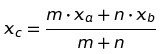
To calculate your interest rate, you need to know the interest formula I/Pt = r to get your rate. Here,

I = Interest amount paid in a specific time period (month, year etc.)

P = Principle amount (the money before interest)

t = Time period involved

r = Interest rate in decimal

You should remember this equation to calculate your basic interest rate.

Step 2

Once you put all the values required to calculate your interest rate, you will get your interest rate in decimal. Now, you need to convert the interest rate you got by multiplying it by 100. For example, a decimal like .11 will not help much while figuring out your interest rate. So, if you want to find your interest rate for .11, you have to multiply .11 with 100 (.11 x 100).

For this case, your interest rate will be (.11 x 100 = 11) 11%.

Step 3

Apart from this, you can also calculate your time period involved, principal amount and interest amount paid in a specific time period if you have other inputs available with you.

Calculate interest amount paid in a specific time period, I = Prt.

Calculate the principal amount, P = I/rt.

Calculate time period involved t = I/Pr.

Step 4

Most importantly, you have to make sure that your time period and interest rate are following the same parameter.

For example, on a loan, you want to find your monthly interest rate after one year. In this case, if you put t = 1, you will get the final interest rate as the interest rate per year. Whereas, if you want the monthly interest rate, you have to put the correct amount of time elapsed. Here, you can consider the time period like 12 months.

Please remember, your time period should be the same time amount as the interest paid. For example, if you’re calculating a year’s monthly interest payments then, it can be considered you’ve made 12 payments.

Also, you have to make sure that you check the time period (weekly, monthly, yearly etc.) when your interest is calculated with your bank.

Step 5

You can rely on online calculators to get interest rates for complex loans, such as mortgages. You should also know the interest rate of your loan when you sign up for it.

For fluctuating rates, sometimes it becomes difficult to determine what a certain rate means. So, it is better to use free online calculators by searching “variable APR interest calculator”, “mortgage interest calculator” etc.

Calculation of interest when rate of interest and cash price is given

  • Where Cash Price, Interest Rate and Instalment are Given:

Illustration:

On 1st January 2003, A bought a television from a seller under Hire Purchase System, the cash price of which being Rs 10.450 as per the following terms:

(a) Rs 3,000 to be paid on signing the agreement.

(b) Balance to be paid in three equal installments of Rs 3,000 at the end of each year,

(c) The rate of interest charged by the seller is 10% per annum.

You are required to calculate the interest paid by the buyer to the seller each year.

Solution:

Note:

  1. there is no time gap between the signing of the agreement and the cash down payment of Rs 3,000 (1.1.2003). Hence no interest is calculated. The entire amount goes to reduce the cash price.
  2. The interest in the last installment is taken at the differential figure of Rs 285.50 (3,000 – 2,714.50).

(2) Where Cash Price and Installments are Given but Rate of Interest is Omitted:

Where the rate of interest is not given and only the cash price and the total payments under hire purchase installments are given, then the total interest paid is the difference between the cash price of the asset and the total amount paid as per the agreement. This interest amount is apportioned in the ratio of amount outstanding at the end of each period.

Illustration:

Mr. A bought a machine under hire purchase agreement, the cash price of the machine being Rs 18,000. As per the terms, the buyer has to pay Rs 4,000 on signing the agreement and the balance in four installments of Rs 4,000 each, payable at the end of each year. Calculate the interest chargeable at the end of each year.

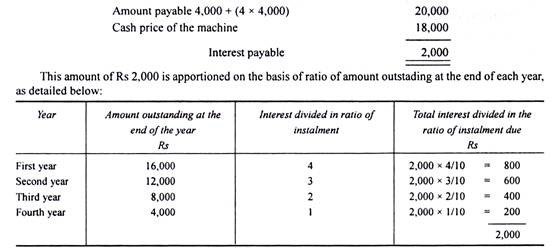
(3) Where installments and Rate of Interest are Given but Cash Value of the Asset is Omitted:

In certain problems, the cash price is not given. It is necessary that we must first find out the cash price and interest included in the installments. The asset account is to be debited with the actual price of the asset. Under such situations, i.e. in the absence of cash price, the interest is calculated from the last year.

It may be noted that the amount of interest goes on increasing from 3rd year to 2nd year, 2nd year to 1st year. Since the interest is included in the installments and by knowing the rate of interest, we can find out the cash price.

Thus:

Let the cash price outstanding be: Rs 100

Interest @ 10% on Rs 100 for a year: Rs 10

Installment paid at the end of the year 110

The interest on installment price = 10/110 or 1/11 as a ratio.
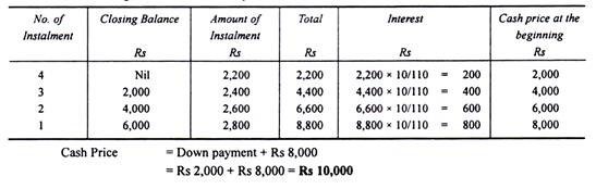
Illustration:

I buy a television on Hire Purchase System.

The terms of payment are as follows:

Rs 2,000 to be paid on signing the agreement;

Rs 2,800 at the end of the first year;

Rs 2,600 at the end of the second year;

Rs 2,400 at the end of the third year;

Rs 2,200 at the end of the fourth year.

If interest is charged at the rate of 10% p.a., what was the cash value of the television?

Solution:

(4) Calculation of Cash Price when Reference to Annuity Table, the Rate of Interest and Installments are Given:

Sometimes in the problem a reference to annuity table wherein present value of the annuity for a number of years at a certain rate of interest is given. In such cases the cash price is calculated by multiplying the amount of installment and adding the product to the initial payment.

Illustration:

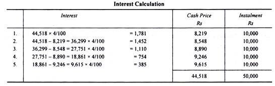
A agrees to purchase a machine from a seller under Hire Purchase System by annual installment of Rs 10,000 over a period of 5 years. The seller charges interest at 4% p.a. on yearly balance.

N.B. The present value of Re 1 p.a. for five years at 4% is Rs 4.4518. Find out the cash price of the machine.

Solution:

Installment Re 1 Present value = Rs 4.4518

Installment = Rs 10,000 Present value = Rs 4.4518 x 10,000 = Rs 44,518

Determinants of the Value of Bonds

Bonds are fixed-income securities that represent a loan from an investor to a borrower, typically a corporation or government. When purchasing a bond, the investor lends money in exchange for periodic interest payments and the return of the bond’s face value at maturity. Bonds are used to finance various projects and operations, providing a predictable income stream for investors.

Valuation of Bonds

The method for valuation of bonds involves three steps as follows:

Step 1: Estimate the expected cash flows

Step 2: Determine the appropriate interest rate that should be used to discount the cash flows.

& Step 3: Calculate the present value of the expected cash flows (step-1) using appropriate interest rate (step- 2) i.e. discounting the expected cash flows

Step 1: Estimating cash flows

Cash flow is the cash that is estimated to be received in future from investment in a bond. There are only two types of cash flows that can be received from investment in bonds i.e. coupon payments and principal payment at maturity.

The usual cash flow cycle of the bond is coupon payments are received at regular intervals as per the bond agreement, and final coupon plus principle payment is received at the maturity. There are some instances when bonds don’t follow these regular patterns. Unusual patterns maybe a result of the different type of bond such as zero-coupon bonds, in which there are no coupon payments. Considering such factors, it is important for an analyst to estimate accurate cash flow for the purpose of bond valuation.

Step 2: Determine the appropriate interest rate to discount the cash flows

Once the cash flow for the bond is estimated, the next step is to determine the appropriate interest rate to discount cash flows. The minimum interest rate that an investor should require is the interest available in the marketplace for default-free cash flow. Default-free cash flows are cash flows from debt security which are completely safe and has zero chances default. Such securities are usually issued by the central bank of a country, for example, in the USA it is bonds by U.S. Treasury Security.

Consider a situation where an investor wants to invest in bonds. If he is considering to invest corporate bonds, he is expecting to earn higher return from these corporate bonds compared to rate of returns of U.S. Treasury Security bonds. This is because chances are that a corporate bond might default, whereas the U.S. Security Treasury bond is never going to default. As he is taking a higher risk by investing in corporate bonds, he expects a higher return.

One may use single interest rate or multiple interest rates for valuation.

Step 3: Discounting the expected cash flows

Now that we already have values of expected future cash flows and interest rate used to discount the cash flow, it is time to find the present value of cash flows. Present Value of a cash flow is the amount of money that must be invested today to generate a specific future value. The present value of a cash flow is more commonly known as discounted value.

The present value of a cash flow depends on two determinants:

  • When a cash flow will be received i.e. timing of a cash flow &;
  • The required interest rate, more widely known as Discount Rate (rate as per Step-2)

First, we calculate the present value of each expected cash flow. Then we add all the individual present values and the resultant sum is the value of the bond.

The formula to find the present value of one cash flow is:

Present value formula for Bond Valuation

Present Value n = Expected cash flow in the period n/ (1+i) n

Here,

i = rate of return/discount rate on bond
n = expected time to receive the cash flow

By this formula, we will get the present value of each individual cash flow t years from now. The next step is to add all individual cash flows.

Bond Value = Present Value 1 + Present Value 2 + ……. + Present Value n

Sampling and Sampling Distribution

Sample design is the framework, or road map, that serves as the basis for the selection of a survey sample and affects many other important aspects of a survey as well. In a broad context, survey researchers are interested in obtaining some type of information through a survey for some population, or universe, of interest. One must define a sampling frame that represents the population of interest, from which a sample is to be drawn. The sampling frame may be identical to the population, or it may be only part of it and is therefore subject to some under coverage, or it may have an indirect relationship to the population.

Sampling is the process of selecting a subset of individuals, items, or observations from a larger population to analyze and draw conclusions about the entire group. It is essential in statistics when studying the entire population is impractical, time-consuming, or costly. Sampling can be done using various methods, such as random, stratified, cluster, or systematic sampling. The main objectives of sampling are to ensure representativeness, reduce costs, and provide timely insights. Proper sampling techniques enhance the reliability and validity of statistical analysis and decision-making processes.

Steps in Sample Design

While developing a sampling design, the researcher must pay attention to the following points:

  • Type of Universe:

The first step in developing any sample design is to clearly define the set of objects, technically called the Universe, to be studied. The universe can be finite or infinite. In finite universe the number of items is certain, but in case of an infinite universe the number of items is infinite, i.e., we cannot have any idea about the total number of items. The population of a city, the number of workers in a factory and the like are examples of finite universes, whereas the number of stars in the sky, listeners of a specific radio programme, throwing of a dice etc. are examples of infinite universes.

  • Sampling unit:

A decision has to be taken concerning a sampling unit before selecting sample. Sampling unit may be a geographical one such as state, district, village, etc., or a construction unit such as house, flat, etc., or it may be a social unit such as family, club, school, etc., or it may be an individual. The researcher will have to decide one or more of such units that he has to select for his study.

  • Source list:

It is also known as ‘sampling frame’ from which sample is to be drawn. It contains the names of all items of a universe (in case of finite universe only). If source list is not available, researcher has to prepare it. Such a list should be comprehensive, correct, reliable and appropriate. It is extremely important for the source list to be as representative of the population as possible.

  • Size of Sample:

This refers to the number of items to be selected from the universe to constitute a sample. This a major problem before a researcher. The size of sample should neither be excessively large, nor too small. It should be optimum. An optimum sample is one which fulfills the requirements of efficiency, representativeness, reliability and flexibility. While deciding the size of sample, researcher must determine the desired precision as also an acceptable confidence level for the estimate. The size of population variance needs to be considered as in case of larger variance usually a bigger sample is needed. The size of population must be kept in view for this also limits the sample size. The parameters of interest in a research study must be kept in view, while deciding the size of the sample. Costs too dictate the size of sample that we can draw. As such, budgetary constraint must invariably be taken into consideration when we decide the sample size.

  • Parameters of interest:

In determining the sample design, one must consider the question of the specific population parameters which are of interest. For instance, we may be interested in estimating the proportion of persons with some characteristic in the population, or we may be interested in knowing some average or the other measure concerning the population. There may also be important sub-groups in the population about whom we would like to make estimates. All this has a strong impact upon the sample design we would accept.

  • Budgetary constraint:

Cost considerations, from practical point of view, have a major impact upon decisions relating to not only the size of the sample but also to the type of sample. This fact can even lead to the use of a non-probability sample.

  • Sampling procedure:

Finally, the researcher must decide the type of sample he will use i.e., he must decide about the technique to be used in selecting the items for the sample. In fact, this technique or procedure stands for the sample design itself. There are several sample designs (explained in the pages that follow) out of which the researcher must choose one for his study. Obviously, he must select that design which, for a given sample size and for a given cost, has a smaller sampling error.

Types of Samples

  • Probability Sampling (Representative samples)

Probability samples are selected in such a way as to be representative of the population. They provide the most valid or credible results because they reflect the characteristics of the population from which they are selected (e.g., residents of a particular community, students at an elementary school, etc.). There are two types of probability samples: random and stratified.

  • Random Sample

The term random has a very precise meaning. Each individual in the population of interest has an equal likelihood of selection. This is a very strict meaning you can’t just collect responses on the street and have a random sample.

The assumption of an equal chance of selection means that sources such as a telephone book or voter registration lists are not adequate for providing a random sample of a community. In both these cases there will be a number of residents whose names are not listed. Telephone surveys get around this problem by random-digit dialling but that assumes that everyone in the population has a telephone. The key to random selection is that there is no bias involved in the selection of the sample. Any variation between the sample characteristics and the population characteristics is only a matter of chance.

  • Stratified Sample

A stratified sample is a mini-reproduction of the population. Before sampling, the population is divided into characteristics of importance for the research. For example, by gender, social class, education level, religion, etc. Then the population is randomly sampled within each category or stratum. If 38% of the population is college-educated, then 38% of the sample is randomly selected from the college-educated population.

Stratified samples are as good as or better than random samples, but they require fairly detailed advance knowledge of the population characteristics, and therefore are more difficult to construct.

  • Non-probability Samples (Non-representative samples)

As they are not truly representative, non-probability samples are less desirable than probability samples. However, a researcher may not be able to obtain a random or stratified sample, or it may be too expensive. A researcher may not care about generalizing to a larger population. The validity of non-probability samples can be increased by trying to approximate random selection, and by eliminating as many sources of bias as possible.

  • Quota Sample

The defining characteristic of a quota sample is that the researcher deliberately sets the proportions of levels or strata within the sample. This is generally done to insure the inclusion of a particular segment of the population. The proportions may or may not differ dramatically from the actual proportion in the population. The researcher sets a quota, independent of population characteristics.

Example: A researcher is interested in the attitudes of members of different religions towards the death penalty. In Iowa a random sample might miss Muslims (because there are not many in that state). To be sure of their inclusion, a researcher could set a quota of 3% Muslim for the sample. However, the sample will no longer be representative of the actual proportions in the population. This may limit generalizing to the state population. But the quota will guarantee that the views of Muslims are represented in the survey.

  • Purposive Sample

A purposive sample is a non-representative subset of some larger population, and is constructed to serve a very specific need or purpose. A researcher may have a specific group in mind, such as high level business executives. It may not be possible to specify the population they would not all be known, and access will be difficult. The researcher will attempt to zero in on the target group, interviewing whoever is available.

  • Convenience Sample

A convenience sample is a matter of taking what you can get. It is an accidental sample. Although selection may be unguided, it probably is not random, using the correct definition of everyone in the population having an equal chance of being selected. Volunteers would constitute a convenience sample.

Non-probability samples are limited with regard to generalization. Because they do not truly represent a population, we cannot make valid inferences about the larger group from which they are drawn. Validity can be increased by approximating random selection as much as possible, and making every attempt to avoid introducing bias into sample selection.

Sampling Distribution

Sampling Distribution is a statistical concept that describes the probability distribution of a given statistic (e.g., mean, variance, or proportion) derived from repeated random samples of a specific size taken from a population. It plays a crucial role in inferential statistics, providing the foundation for making predictions and drawing conclusions about a population based on sample data.

Concepts of Sampling Distribution

A sampling distribution is the distribution of a statistic (not raw data) over all possible samples of the same size from a population. Commonly used statistics include the sample mean (Xˉ\bar{X}), sample variance, and sample proportion.

Purpose:

It allows statisticians to estimate population parameters, test hypotheses, and calculate probabilities for statistical inference.

Shape and Characteristics:

    • The shape of the sampling distribution depends on the population distribution and the sample size.
    • For large sample sizes, the Central Limit Theorem states that the sampling distribution of the mean will be approximately normal, regardless of the population’s distribution.

Importance of Sampling Distribution

  • Facilitates Statistical Inference:

Sampling distributions are used to construct confidence intervals and perform hypothesis tests, helping to infer population characteristics.

  • Standard Error:

The standard deviation of the sampling distribution, called the standard error, quantifies the variability of the sample statistic. Smaller standard errors indicate more reliable estimates.

  • Links Population and Samples:

It provides a theoretical framework that connects sample statistics to population parameters.

Types of Sampling Distributions

  • Distribution of Sample Means:

Shows the distribution of means from all possible samples of a population.

  • Distribution of Sample Proportions:

Represents the proportion of a certain outcome in samples, used in binomial settings.

  • Distribution of Sample Variances:

Explains the variability in sample data.

Example

Consider a population of students’ test scores with a mean of 70 and a standard deviation of 10. If we repeatedly draw random samples of size 30 and calculate the sample mean, the distribution of those means forms the sampling distribution. This distribution will have a mean close to 70 and a reduced standard deviation (standard error).

Present Value, Functions

Present Value (PV) concept refers to the current worth of a future sum of money or stream of cash flows, discounted at a specific interest rate. It reflects the principle that a dollar today is worth more than a dollar in the future due to its potential earning capacity.

PV = FV / (1+r)^n

where

FV is the future value,

r is the discount rate,

n is the number of periods until payment.

This concept is essential in finance for assessing investment opportunities and financial planning.

Functions of Present Value:

  • Valuation of Cash Flows:

PV allows investors and analysts to evaluate the worth of future cash flows generated by an investment. By discounting future cash flows to their present value, stakeholders can determine if the investment is financially viable compared to its cost.

  • Investment Decision Making:

In capital budgeting, PV is crucial for assessing whether to proceed with projects or investments. By comparing the present value of expected cash inflows to the initial investment (cost), decision-makers can prioritize projects that offer the highest returns relative to their costs.

  • Comparison of Investment Alternatives:

PV provides a standardized method for comparing different investment opportunities. By converting future cash flows into their present values, investors can effectively evaluate and contrast various investments, regardless of their cash flow patterns or timing.

  • Financial Planning:

Individuals and businesses use PV for financial planning and retirement savings. By calculating the present value of future financial goals (like retirement funds), individuals can determine how much they need to save and invest today to achieve those goals.

  • Debt Valuation:

PV is essential for valuing bonds and other debt instruments. The present value of future interest payments and the principal repayment is calculated to determine the fair market value of the bond. This valuation helps investors make informed decisions about purchasing or selling bonds.

  • Risk Assessment:

Present Value helps in assessing the risk associated with investments. Higher discount rates, which account for risk and uncertainty, lower the present value of future cash flows. This relationship allows investors to gauge the risk-return trade-off of different investments effectively.

Present Value of a Single Flow:

Used when we have a single future amount to be received after a certain time.

Formula:

Example:

You will receive ₹15,000 after 3 years. What is its present value if the discount rate is 10%?

Future Value () Years Rate (%) PV ()
15,000 3 10 11,270

This applies when cash flows are not equal each year. Each amount is discounted separately.

Present Value of Uneven Cash Flows

Example:

You will receive ₹2,000 in Year 1, ₹3,000 in Year 2, and ₹4,000 in Year 3. Discount rate = 10%

Year Cash Flow () PV Factor @10% Present Value ()
1 2,000 0.909 1,818
2 3,000 0.826 2,478
3 4,000 0.751 3,004
₹7,300

Present Value of an Annuity (Ordinary Annuity):

Used when you receive equal payments at the end of each period for a specific number of years.

Present Value of an Annuity (Ordinary Annuity)

Example:

You will receive ₹2,000 every year for 3 years. Discount rate = 10%

PV = 2,000 × (1−(1+0.10)^−3 / 0.10) = 2,000 × 2.487 = ₹4,974

Year Payment ()

PV Factor @10%

PV ()
1 2,000 0.909 1,818
2 2,000 0.826 1,652
3 2,000 0.751 1,504

4,974

Future Value, Functions, Types

Future Value (FV) is the value of a current asset at a future date based on an assumed rate of growth. The future value (FV) is important to investors and financial planners as they use it to estimate how much an investment made today will be worth in the future. Knowing the future value enables investors to make sound investment decisions based on their anticipated needs.

FV calculation allows investors to predict, with varying degrees of accuracy, the amount of profit that can be generated by different investments. The amount of growth generated by holding a given amount in cash will likely be different than if that same amount were invested in stocks; so, the FV equation is used to compare multiple options.

Determining the FV of an asset can become complicated, depending on the type of asset. Also, the FV calculation is based on the assumption of a stable growth rate. If money is placed in a savings account with a guaranteed interest rate, then the FV is easy to determine accurately. However, investments in the stock market or other securities with a more volatile rate of return can present greater difficulty.

Future Value (FV) formula assumes a constant rate of growth and a single upfront payment left untouched for the duration of the investment. The FV calculation can be done one of two ways depending on the type of interest being earned. If an investment earns simple interest, then the Future Value (FV) formula is:

  • Future value (FV) is the value of a current asset at some point in the future based on an assumed growth rate.
  • Investors are able to reasonably assume an investment’s profit using the future value (FV) calculation.
  • Determining the future value (FV) of a market investment can be challenging because of the market’s volatility.
  • There are two ways of calculating the future value (FV) of an asset: FV using simple interest and FV using compound interest.

Functions of Future Value:

  • Investment Growth Measurement:

FV is used to calculate how much an investment will grow over time. By applying a specified interest rate, investors can estimate the future worth of their initial investments or savings, helping them understand the potential returns.

  • Retirement Planning:

FV plays a critical role in retirement planning. Individuals can determine how much they need to save today to achieve a desired retirement income. By calculating the future value of regular contributions to retirement accounts, they can set realistic savings goals.

  • Loan Repayment Calculations:

For borrowers, FV is crucial in understanding the total amount owed on loans over time. It helps them visualize the long-term cost of borrowing, including interest payments, aiding in budgeting and financial decision-making.

  • Comparison of Investment Opportunities:

FV provides a standardized way to compare different investment options. By calculating the future value of various investment opportunities, investors can evaluate which options offer the highest potential returns over a specified period.

  • Education Funding:

Parents can use FV to plan for their children’s education expenses. By estimating future tuition costs and calculating how much they need to save now, parents can ensure they accumulate sufficient funds by the time their children enter college.

  • Inflation Adjustment:

FV helps investors account for inflation when planning for future expenses. By incorporating an expected inflation rate into future value calculations, individuals and businesses can better estimate the amount needed to maintain purchasing power over time.

Future Value of a Single Flow:

This occurs when a single sum of money is invested for a certain period at a given interest rate.

Formula:

FV = PV × (1+r)^n

Example:

Suppose ₹10,000 is invested for 3 years at 10% annual interest.

Year Calculation Future Value ()

3

₹10,000 × (1 + 0.10)^3

₹13,310

Range and co-efficient of Range

The range is a measure of dispersion that represents the difference between the highest and lowest values in a dataset. It provides a simple way to understand the spread of data. While easy to calculate, the range is sensitive to outliers and does not provide information about the distribution of values between the extremes.

Range of a distribution gives a measure of the width (or the spread) of the data values of the corresponding random variable. For example, if there are two random variables X and Y such that X corresponds to the age of human beings and Y corresponds to the age of turtles, we know from our general knowledge that the variable corresponding to the age of turtles should be larger.

Since the average age of humans is 50-60 years, while that of turtles is about 150-200 years; the values taken by the random variable Y are indeed spread out from 0 to at least 250 and above; while those of X will have a smaller range. Thus, qualitatively you’ve already understood what the Range of a distribution means. The mathematical formula for the same is given as:

Range = L – S

where

L: The Largets/maximum value attained by the random variable under consideration

S: The smallest/minimum value.

Properties

  • The Range of a given distribution has the same units as the data points.
  • If a random variable is transformed into a new random variable by a change of scale and a shift of origin as:

Y = aX + b

where

Y: the new random variable

X: the original random variable

a,b: constants.

Then the ranges of X and Y can be related as:

RY = |a|RX

Clearly, the shift in origin doesn’t affect the shape of the distribution, and therefore its spread (or the width) remains unchanged. Only the scaling factor is important.

  • For a grouped class distribution, the Range is defined as the difference between the two extreme class boundaries.
  • A better measure of the spread of a distribution is the Coefficient of Range, given by:

Coefficient of Range (expressed as a percentage) = L – SL + S × 100

Clearly, we need to take the ratio between the Range and the total (combined) extent of the distribution. Besides, since it is a ratio, it is dimensionless, and can, therefore, one can use it to compare the spreads of two or more different distributions as well.

  • The range is an absolute measure of Dispersion of a distribution while the Coefficient of Range is a relative measure of dispersion.

Due to the consideration of only the end-points of a distribution, the Range never gives us any information about the shape of the distribution curve between the extreme points. Thus, we must move on to better measures of dispersion. One such quantity is Mean Deviation which is we are going to discuss now.

Interquartile range (IQR)

The interquartile range is the middle half of the data. To visualize it, think about the median value that splits the dataset in half. Similarly, you can divide the data into quarters. Statisticians refer to these quarters as quartiles and denote them from low to high as Q1, Q2, Q3, and Q4. The lowest quartile (Q1) contains the quarter of the dataset with the smallest values. The upper quartile (Q4) contains the quarter of the dataset with the highest values. The interquartile range is the middle half of the data that is in between the upper and lower quartiles. In other words, the interquartile range includes the 50% of data points that fall in Q2 and

The IQR is the red area in the graph below.

The interquartile range is a robust measure of variability in a similar manner that the median is a robust measure of central tendency. Neither measure is influenced dramatically by outliers because they don’t depend on every value. Additionally, the interquartile range is excellent for skewed distributions, just like the median. As you’ll learn, when you have a normal distribution, the standard deviation tells you the percentage of observations that fall specific distances from the mean. However, this doesn’t work for skewed distributions, and the IQR is a great alternative.

I’ve divided the dataset below into quartiles. The interquartile range (IQR) extends from the low end of Q2 to the upper limit of Q3. For this dataset, the range is 21 – 39.

Skewness

Skewness, in statistics, is the degree of distortion from the symmetrical bell curve, or normal distribution, in a set of data. Skewness can be negative, positive, zero or undefined. A normal distribution has a skew of zero, while a lognormal distribution, for example, would exhibit some degree of right-skew.

The three probability distributions depicted below depict increasing levels of right (or positive) skewness. Distributions can also be left (negative) skewed. Skewness is used along with kurtosis to better judge the likelihood of events falling in the tails of a probability distribution.

Right skewness

  • Skewness, in statistics, is the degree of distortion from the symmetrical bell curve in a probability distribution.
  • Distributions can exhibit right (positive) skewness or left (negative) skewness to varying degree.
  • Investors note skewness when judging a return distribution because it, like kurtosis, considers the extremes of the data set rather than focusing solely on the average.

Broadly speaking, there are two types of skewness: They are

(1) Positive skewness

(2) Negative skewnes.

Positive skewness

A series is said to have positive skewness when the following characteristics are noticed:

  • Mean > Median > Mode.
  • The right tail of the curve is longer than its left tail, when the data are plotted through a histogram, or a frequency polygon.
  • The formula of Skewness and its coefficient give positive figures.

Negative Skewness

A series is said to have negative skewness when the following characteristics are noticed:

  • Mode> Median > Mode.
  • The left tail of the curve is longer than the right tail, when the data are plotted through a histogram, or a frequency polygon.
  • The formula of skewness and its coefficient give negative figures.

Thus, a statistical distribution may be three types viz.

  • Symmetric
  • Positively skewed
  • Negatively skewed

Skewness Co-efficient

  1. Pearson’s Coefficient of Skewness #1 uses the mode. The formula is:

    pearson skewness

    Where xbar = the mean, Mo = the mode and s = the standard deviation for the sample.

  2. Pearson’s Coefficient of Skewness #2 uses the median. The formula is:

    Pearson's Coefficient of Skewness

    Where xbar = the mean, Mo = the mode and s = the standard deviation for the sample.

    It is generally used when you don’t know the mode.

Karl Pearson and Rank co-relation

Karl Pearson Coefficient of Correlation (also called the Pearson correlation coefficient or Pearson’s r) is a measure of the strength and direction of the linear relationship between two variables. It ranges from -1 to +1, where +1 indicates a perfect positive linear relationship, -1 indicates a perfect negative linear relationship, and 0 indicates no linear relationship. The formula for Pearson’s r is calculated by dividing the covariance of the two variables by the product of their standard deviations. It is widely used in statistics to analyze the degree of correlation between paired data.

The following are the main properties of correlation.

  1. Coefficient of Correlation lies between -1 and +1:

The coefficient of correlation cannot take value less than -1 or more than one +1. Symbolically,

-1<=r<= + 1 or | r | <1.

  1. Coefficients of Correlation are independent of Change of Origin:

This property reveals that if we subtract any constant from all the values of X and Y, it will not affect the coefficient of correlation.

  1. Coefficients of Correlation possess the property of symmetry:

The degree of relationship between two variables is symmetric as shown below:

  1. Coefficient of Correlation is independent of Change of Scale:

This property reveals that if we divide or multiply all the values of X and Y, it will not affect the coefficient of correlation.

  1. Co-efficient of correlation measures only linear correlation between X and Y.
  2. If two variables X and Y are independent, coefficient of correlation between them will be zero.

Karl Pearson’s Coefficient of Correlation is widely used mathematical method wherein the numerical expression is used to calculate the degree and direction of the relationship between linear related variables.

Pearson’s method, popularly known as a Pearsonian Coefficient of Correlation, is the most extensively used quantitative methods in practice. The coefficient of correlation is denoted by “r”.

If the relationship between two variables X and Y is to be ascertained, then the following formula is used:

Properties of Coefficient of Correlation

  • The value of the coefficient of correlation (r) always lies between±1. Such as:

    r=+1, perfect positive correlation

    r=-1, perfect negative correlation

    r=0, no correlation

  • The coefficient of correlation is independent of the origin and scale.By origin, it means subtracting any non-zero constant from the given value of X and Y the vale of “r” remains unchanged. By scale it means, there is no effect on the value of “r” if the value of X and Y is divided or multiplied by any constant.
  • The coefficient of correlation is a geometric mean of two regression coefficient. Symbolically it is represented as:
  • The coefficient of correlation is “ zero” when the variables X and Y are independent. But, however, the converse is not true.

Assumptions of Karl Pearson’s Coefficient of Correlation

  1. The relationship between the variables is “Linear”, which means when the two variables are plotted, a straight line is formed by the points plotted.
  2. There are a large number of independent causes that affect the variables under study so as to form a Normal Distribution. Such as, variables like price, demand, supply, etc. are affected by such factors that the normal distribution is formed.
  3. The variables are independent of each other.                                     

Note: The coefficient of correlation measures not only the magnitude of correlation but also tells the direction. Such as, r = -0.67, which shows correlation is negative because the sign is “-“ and the magnitude is 0.67.

Spearman Rank Correlation

Spearman rank correlation is a non-parametric test that is used to measure the degree of association between two variables.  The Spearman rank correlation test does not carry any assumptions about the distribution of the data and is the appropriate correlation analysis when the variables are measured on a scale that is at least ordinal.

The Spearman correlation between two variables is equal to the Pearson correlation between the rank values of those two variables; while Pearson’s correlation assesses linear relationships, Spearman’s correlation assesses monotonic relationships (whether linear or not). If there are no repeated data values, a perfect Spearman correlation of +1 or −1 occurs when each of the variables is a perfect monotone function of the other.

Intuitively, the Spearman correlation between two variables will be high when observations have a similar (or identical for a correlation of 1) rank (i.e. relative position label of the observations within the variable: 1st, 2nd, 3rd, etc.) between the two variables, and low when observations have a dissimilar (or fully opposed for a correlation of −1) rank between the two variables.

The following formula is used to calculate the Spearman rank correlation:

ρ = Spearman rank correlation

di = the difference between the ranks of corresponding variables

n = number of observations

Assumptions

The assumptions of the Spearman correlation are that data must be at least ordinal and the scores on one variable must be monotonically related to the other variable.

Data Tabulation

Tabulation is the systematic arrangement of the statistical data in columns or rows. It involves the orderly and systematic presentation of numerical data in a form designed to explain the problem under consideration. Tabulation helps in drawing the inference from the statistical figures.

Tabulation prepares the ground for analysis and interpretation. Therefore a suitable method must be decided carefully taking into account the scope and objects of the investigation, because it is very important part of the statistical methods.

Types of Tabulation

In general, the tabulation is classified in two parts, that is a simple tabulation, and a complex tabulation.

Simple tabulation, gives information regarding one or more independent questions. Complex tabulation gives information regarding two mutually dependent questions.

  • Two-Way Table

These types of table give information regarding two mutually dependent questions. For example, question is, how many millions of the persons are in the Divisions; the One-Way Table will give the answer. But if we want to know that in the population number, who are in the majority, male, or female. The Two-Way Tables will answer the question by giving the column for female and male. Thus the table showing the real picture of divisions sex wise is as under:

  • Three-Way Table

Three-Way Table gives information regarding three mutually dependent and inter-related questions.

For example, from one-way table, we get information about population, and from two-way table, we get information about the number of male and female available in various divisions. Now we can extend the same table to a three way table, by putting a question, “How many male and female are literate?” Thus the collected statistical data will show the following, three mutually dependent and inter-related questions:

  1. Population in various division.
  2. Their sex-wise distribution.
  3. Their position of literacy.

Presentation of Data

Presentation of data is of utter importance nowadays. Afterall everything that’s pleasing to our eyes never fails to grab our attention. Presentation of data refers to an exhibition or putting up data in an attractive and useful manner such that it can be easily interpreted. The three main forms of presentation of data are:

  1. Textual presentation
  2. Data tables
  3. Diagrammatic presentation

Textual Presentation

The discussion about the presentation of data starts off with it’s most raw and vague form which is the textual presentation. In such form of presentation, data is simply mentioned as mere text, that is generally in a paragraph. This is commonly used when the data is not very large.

This kind of representation is useful when we are looking to supplement qualitative statements with some data. For this purpose, the data should not be voluminously represented in tables or diagrams. It just has to be a statement that serves as a fitting evidence to our qualitative evidence and helps the reader to get an idea of the scale of a phenomenon.

For example, “the 2002 earthquake proved to be a mass murderer of humans. As many as 10,000 citizens have been reported dead”. The textual representation of data simply requires some intensive reading. This is because the quantitative statement just serves as an evidence of the qualitative statements and one has to go through the entire text before concluding anything.

Further, if the data under consideration is large then the text matter increases substantially. As a result, the reading process becomes more intensive, time-consuming and cumbersome.

Data Tables or Tabular Presentation

A table facilitates representation of even large amounts of data in an attractive, easy to read and organized manner. The data is organized in rows and columns. This is one of the most widely used forms of presentation of data since data tables are easy to construct and read.

Components of Data Tables

  • Table Number: Each table should have a specific table number for ease of access and locating. This number can be readily mentioned anywhere which serves as a reference and leads us directly to the data mentioned in that particular table.
  • Title: A table must contain a title that clearly tells the readers about the data it contains, time period of study, place of study and the nature of classification of data.
  • Headnotes: A headnote further aids in the purpose of a title and displays more information about the table. Generally, headnotes present the units of data in brackets at the end of a table title.
  • Stubs: These are titles of the rows in a table. Thus a stub display information about the data contained in a particular row.
  • Caption: A caption is the title of a column in the data table. In fact, it is a counterpart if a stub and indicates the information contained in a column.
  • Body or field: The body of a table is the content of a table in its entirety. Each item in a body is known as a ‘cell’.
  • Footnotes: Footnotes are rarely used. In effect, they supplement the title of a table if required.
  • Source: When using data obtained from a secondary source, this source has to be mentioned below the footnote.

Construction of Data Tables

There are many ways for construction of a good table. However, some basic ideas are:

  • The title should be in accordance with the objective of study: The title of a table should provide a quick insight into the table.
  • Comparison: If there might arise a need to compare any two rows or columns then these might be kept close to each other.
  • Alternative location of stubs: If the rows in a data table are lengthy, then the stubs can be placed on the right-hand side of the table.
  • Headings: Headings should be written in a singular form. For example, ‘good’ must be used instead of ‘goods’.
  • Footnote: A footnote should be given only if needed.
  • Size of columns: Size of columns must be uniform and symmetrical.
  • Use of abbreviations: Headings and sub-headings should be free of abbreviations.
  • Units: There should be a clear specification of units above the columns.

Advantages of Tabular Presentation:

  • Ease of representation: A large amount of data can be easily confined in a data table. Evidently, it is the simplest form of data presentation.
  • Ease of analysis: Data tables are frequently used for statistical analysis like calculation of central tendency, dispersion etc.
  • Helps in comparison: In a data table, the rows and columns which are required to be compared can be placed next to each other. To point out, this facilitates comparison as it becomes easy to compare each value.
  • Economical: Construction of a data table is fairly easy and presents the data in a manner which is really easy on the eyes of a reader. Moreover, it saves time as well as space.

Classification of Data and Tabular Presentation

Qualitative Classification

In this classification, data in a table is classified on the basis of qualitative attributes. In other words, if the data contained attributes that cannot be quantified like rural-urban, boys-girls etc. it can be identified as a qualitative classification of data.

Sex Urban Rural
Boys 200 390
Girls 167 100

Quantitative Classification

In quantitative classification, data is classified on basis of quantitative attributes.

Marks No. of Students
0-50 29
51-100 64

Temporal Classification

Here data is classified according to time. Thus when data is mentioned with respect to different time frames, we term such a classification as temporal.

Year Sales
2016 10,000
2017 12,500

Spatial Classification

When data is classified according to a location, it becomes a spatial classification.

Country No. of Teachers
India 139,000
Russia 43,000

Advantages of Tabulation

  1. The large mass of confusing data is easily reduced to reasonable form that is understandable to kind.
  2. The data once arranged in a suitable form, gives the condition of the situation at a glance, or gives a bird eye view.
  3. From the table it is easy to draw some reasonable conclusion or inferences.
  4. Tables gave grounds for analysis of the data.
  5. Errors, and omission if any are always detected in tabulation.

Mean (AM, Weighted, Combined)

Arithmetic Mean

The arithmetic mean,’ mean or average is calculated by summ­ing all the individual observations or items of a sample and divid­ing this sum by the number of items in the sample. For example, as the result of a gas analysis in a respirometer an investigator obtains the following four readings of oxygen percentages:

14.9
10.8
12.3
23.3
Sum = 61.3

He calculates the mean oxygen percentage as the sum of the four items divided by the number of items here, by four. Thus, the average oxygen percentage is

Mean = 61.3 / 4 =15.325%

Calculating a mean presents us with the opportunity for learning statistical symbolism. An individual observation is symbo­lized by Yi, which stands for the ith observation in the sample. Four observations could be written symbolically as Yi, Y2, Y3, Y4.

We shall define n, the sample size, as the number of items in a sample. In this particular instance, the sample size n is 4. Thus, in a large sample, we can symbolize the array from the first to the nth item as follows: Y1, Y2…, Yn. When we wish to sum items, we use the following notation:

The capital Greek sigma, Ʃ, simply means the sum of items indica­ted. The i = 1 means that the items should be summed, starting with the first one, and ending with the nth one as indicated by the i = n above the Ʃ. The subscript and superscript are necessary to indicate how many items should be summed. Below are seen increasing simplifications of the complete notation shown at the extreme left:

Properties of Arithmetic Mean:

  1. The sum of deviations of the items from the arithmetic mean is always zero i.e.

∑(X–X) =0.

  1. The Sum of the squared deviations of the items from A.M. is minimum, which is less than the sum of the squared deviations of the items from any other values.
  2. If each item in the series is replaced by the mean, then the sum of these substitutions will be equal to the sum of the individual items.                       

Merits of A.M:

  1. It is simple to understand and easy to calculate.
  2. It is affected by the value of every item in the series.
  3. It is rigidly defined.
  4. It is capable of further algebraic treatment.
  5. It is calculated value and not based on the position in the series.

Demerits of A.M:

  1. It is affected by extreme items i.e., very small and very large items.
  2. It can hardly be located by inspection.
  3. In some cases A.M. does not represent the actual item. For example, average patients admitted in a hospital is 10.7 per day.
  4. M. is not suitable in extremely asymmetrical distributions.

Weighted Mean

In some cases, you might want a number to have more weight. In that case, you’ll want to find the weighted mean. To find the weighted mean:

  1. Multiply the numbers in your data set by the weights.
  2. Add the results up.

For that set of number above with equal weights (1/5 for each number), the math to find the weighted mean would be:
1(*1/5) + 3(*1/5) + 5(*1/5) + 7(*1/5) + 10(*1/5) = 5.2.

Sample problem: You take three 100-point exams in your statistics class and score 80, 80 and 95. The last exam is much easier than the first two, so your professor has given it less weight. The weights for the three exams are:

  • Exam 1: 40 % of your grade. (Note: 40% as a decimal is .4.)
  • Exam 2: 40 % of your grade.
  • Exam 3: 20 % of your grade.

What is your final weighted average for the class?

  1. Multiply the numbers in your data set by the weights:

    .4(80) = 32

    .4(80) = 32

    .2(95) = 19

  2. Add the numbers up. 32 + 32 + 19 = 83.

The percent weight given to each exam is called a weighting factor.

Weighted Mean Formula

The weighted mean is relatively easy to find. But in some cases the weights might not add up to 1. In those cases, you’ll need to use the weighted mean formula. The only difference between the formula and the steps above is that you divide by the sum of all the weights.

The image above is the technical formula for the weighted mean. In simple terms, the formula can be written as:

Weighted mean = Σwx / Σw

Σ = the sum of (in other words…add them up!).
w = the weights.
x = the value.

To use the formula:

  1. Multiply the numbers in your data set by the weights.
  2. Add the numbers in Step 1 up. Set this number aside for a moment.
  3. Add up all of the weights.
  4. Divide the numbers you found in Step 2 by the number you found in Step 3.

In the sample grades problem above, all of the weights add up to 1 (.4 + .4 + .2) so you would divide your answer (83) by 1:
83 / 1 = 83.

However, let’s say your weighted means added up to 1.2 instead of 1. You’d divide 83 by 1.2 to get:
83 / 1.2 = 69.17.

Combined Mean

A combined mean is a mean of two or more separate groups, and is found by:

  1. Calculating the mean of each group,
  2. Combining the results.

Combined Mean Formula

More formally, a combined mean for two sets can be calculated by the formula :

Where:

  • xa = the mean of the first set,
  • m = the number of items in the first set,
  • xb = the mean of the second set,
  • n = the number of items in the second set,
  • xc the combined mean.

A combined mean is simply a weighted mean, where the weights are the size of each group.

error: Content is protected !!