Tag: Financial Management BU BBA 4th Semester NEP Notes

Relational Logistic Regression is an extension of the traditional logistic regression model designed to handle scenarios where the data exhibits relational or network structures. In many real-world applications, data is not independent and identically distributed; instead, it forms complex relationships or dependencies, such as those found in social networks, communication networks, or biological networks. Relational Logistic Regression is specifically tailored to model the influence of network connections on the binary outcome of interest, making it particularly suitable for tasks like link prediction, community detection, or classification in network-structured data.

Relational Logistic Regression provides a valuable framework for modeling dependencies in network-structured data. By explicitly incorporating node and edge features, it addresses the challenges posed by relational dependencies and is applicable to various domains, including social network analysis, link prediction, and collaborative filtering. As research in this field progresses, the integration of advanced techniques and the exploration of new applications are likely to enhance the capabilities of Relational Logistic Regression in capturing and leveraging relational information for improved predictions.

Concepts of Relational Logistic Regression:

1. Graph Representation:

• Nodes and Edges: The data is structured as a graph, where entities are represented as nodes, and relationships or interactions between entities are represented as edges. This graph captures the relational information in the data.

2. Binary Classification:

• Outcome Variable: The task typically involves binary classification, where each node in the graph is associated with a binary outcome variable, such as the presence or absence of a particular event or link.

3. Relational Features:

• Node Features: Each node is associated with features that describe its attributes.
• Edge Features: In relational logistic regression, the model considers features associated with edges, capturing the characteristics of the relationships between nodes.

4. Influence from Neighbors:

• Neighbor Nodes: The model accounts for the influence of neighboring nodes in the graph on the target node’s outcome. The idea is that the outcome of a node is influenced by the outcomes of its connected neighbors.

5. Parameter Estimation:

• Logistic Regression Coefficients: The model estimates logistic regression coefficients for both node features and edge features. These coefficients quantify the impact of features on the log-odds of the binary outcome.

Relational Logistic Regression Model:

The Relational Logistic Regression model is an extension of the traditional logistic regression model, incorporating relational features and considering dependencies among observations. The logistic regression equation is modified to include terms related to both node features and edge features. The model can be expressed as follows:

Where:

• log-oddslog-odds is the logarithm of the odds of the binary outcome.
• β0​ is the intercept term.
• βi​ are the coefficients associated with node features xi​.
• γj​ are the coefficients associated with edge features yj​.
• p is the number of node features.
• q is the number of edge features.

The logistic function is then applied to the log-odds to obtain the probability of the positive class:

Model Learning and Inference:

1. Model Training:

• Parameter Estimation: The logistic regression coefficients (βi​ and γj​) are estimated through the maximization of the likelihood function using methods like maximum likelihood estimation (MLE) or stochastic gradient descent.

2. Inference and Prediction:

• Probabilistic Predictions: Given the learned coefficients, the model can make probabilistic predictions for the positive class. The predicted probability P(Y=1) is obtained using the logistic function.

• Thresholding for Binary Classification: A threshold is applied to the predicted probability to classify instances into the positive or negative class.

Advantages of Relational Logistic Regression:

1. Accounting for Network Dependencies:

Relational Logistic Regression explicitly models dependencies among entities in a network, making it suitable for scenarios where outcomes are influenced by relational information.

2. Interpretability:

The coefficients associated with node and edge features provide interpretability, allowing practitioners to understand the impact of different features on the binary outcome.

3. Flexible Modeling:

The model is flexible and can be adapted to different types of networks and relational structures, making it applicable to a wide range of scenarios.

Challenges and Considerations:

1. Computational Complexity:

Learning the parameters of Relational Logistic Regression may be computationally intensive, especially for large networks. Efficient optimization algorithms are crucial.

2. Choice of Features:

The selection of relevant node and edge features requires careful consideration. Incorrect or irrelevant features may lead to suboptimal model performance.

3. Handling Imbalanced Data:

If the binary outcome is imbalanced (i.e., one class is much more prevalent than the other), the model may need to be adjusted or evaluated using metrics that account for class imbalance.

Applications of Relational Logistic Regression:

1. Link Prediction:

Predicting the likelihood of a connection between two nodes in a network.

2. Community Detection:

Identifying groups or communities of nodes based on their connectivity patterns.

3. Classification in Social Networks:

Classifying nodes in a social network based on their attributes and connections.

4. Collaborative Filtering:

Predicting user preferences or item recommendations in collaborative filtering scenarios.

Future Directions:

1. Integration with Graph Neural Networks (GNNs):

Combining the strengths of Relational Logistic Regression with the expressive power of GNNs for more effective modeling of relational data.

2. Handling Temporal Networks:

Extending the model to handle temporal dependencies in evolving networks.

3. Advanced Regularization Techniques:

Exploring regularization techniques to enhance model generalization, especially in scenarios with limited labeled data.

Relational Neighbor Classifier (RNC) is a machine learning algorithm that falls under the category of relational learning or inductive logic programming. It’s designed to handle classification tasks in relational or graph-structured data, such as social networks, biological networks, or knowledge graphs. The key idea behind the Relational Neighbor Classifier is to exploit the relational information among entities in a graph to improve classification accuracy.

The Relational Neighbor Classifier is a versatile approach for handling classification tasks in graph-structured data. Its effectiveness lies in its ability to exploit the relational information present in the graph, making it particularly suitable for applications involving interconnected entities.

Components of Relational Neighbor Classifier:

1. Relational Representation:

Graph Structure: The data is represented as a graph where entities are nodes, and relationships are edges. This graph structure captures the relational information in the data.

2. Relational Features:

• Node Features: Each node in the graph has associated features. These features can include attributes of the entity and information derived from its neighbors.
• Edge Features: For edges in the graph, additional features may be considered, representing the strength or type of the relationship.

3. Relational Learning:

• Neighbor Information: The key idea is to leverage information from the neighbors of a node for classification. The assumption is that the class of a node is influenced by the classes of its neighbors.
• Label Propagation: The algorithm may propagate labels or information from neighboring nodes to the target node, considering the relationships in the graph.

4. Classification Model:

• Classifier Type: The underlying classifier can be any traditional classification algorithm, such as decision trees, support vector machines, or logistic regression.
• Integration of Relational Information: The classifier is extended or modified to incorporate relational features and the influence of neighboring nodes.

5. Inference:

Prediction: Given a new or unlabeled node, the model predicts its class based on the learned relational features and the information propagated from neighboring nodes.

Workflow of Relational Neighbor Classifier:

• Graph Representation:

The data is structured as a graph where entities are nodes, and relationships are edges. Each node is associated with features, and the graph captures the relational information among entities.

• Feature Extraction:

Features are extracted for each node and edge in the graph. These features can include attributes of the entities, edge weights, and aggregated information from neighboring nodes.

• Learning Relational Features:

The model learns to capture the relational information by considering the features of a node and its neighbors. This learning process may involve label propagation or other methods to incorporate information from neighboring nodes.

• Classifier Training:

The relational features are used to train a traditional classification model. The classifier is trained to predict the class labels of nodes based on their features and the relational information in the graph.

• Prediction:

When presented with a new or unlabeled node, the classifier utilizes the learned relational features and information from neighboring nodes to predict the class label of the target node.

Advantages of Relational Neighbor Classifier:

• Exploiting Relationships:

RNC leverages the relationships in the graph, allowing it to capture dependencies and influences between entities in the classification process.

• Handling Heterogeneous Data:

RNC is suitable for scenarios where the data is heterogeneous and can be represented as a graph, such as social networks or knowledge graphs.

• Semi–Supervised Learning:

RNC can benefit from semi-supervised learning scenarios where only a subset of nodes in the graph have labeled data. Information from labeled nodes can be propagated to unlabeled nodes.

Challenges and Considerations:

• Scalability:

The performance of RNC can be affected by the size and complexity of the graph. Efficient algorithms for label propagation and feature extraction are crucial.

• Model Interpretability:

As with many complex models, interpretability can be a challenge. Understanding how the model uses relational information for classification is important, especially in applications where interpretability is critical.

• Handling Noisy or Incomplete Data:

RNC may be sensitive to noise or missing information in the graph. Robust methods are needed to handle such scenarios.

Applications:

• Social Network Analysis:

Identifying communities, predicting user preferences, or detecting anomalies in social networks.

• Biological Networks:

Predicting protein functions, identifying gene-disease associations, or classifying biological entities in molecular networks.

• Knowledge Graphs:

Classifying entities in a knowledge graph, such as predicting the category of entities or relationships.

• Recommendation Systems:

Incorporating relational information for personalized recommendations in collaborative filtering scenarios.

Probabilistic Relational Neighbor Classifier, Components, Workflow, Advantages, Challenges, Applications

The Probabilistic Relational Neighbor Classifier (PRNC) is an extension of the Relational Neighbor Classifier (RNC) that incorporates probabilistic modeling into the learning process. Similar to the RNC, the PRNC is designed for classification tasks on graph-structured data, where entities are represented as nodes, relationships as edges, and relational information among entities is crucial for accurate predictions.

The Probabilistic Relational Neighbor Classifier is a sophisticated approach that combines the strengths of probabilistic modeling with relational learning. It is particularly useful in scenarios where uncertainty is inherent in the data and where a probabilistic view of predictions is valuable for decision-making.

Components of Probabilistic Relational Neighbor Classifier:

1. Graph Representation:

• Graph Structure:

The data is modeled as a graph, where nodes represent entities, and edges represent relationships between entities. This graph structure captures the relational information among entities.

2. Probabilistic Graphical Model:

• Graphical Representation:

PRNC utilizes a probabilistic graphical model to represent the joint probability distribution over the nodes in the graph. This model captures dependencies between nodes and incorporates uncertainty in the relationships.

3. Relational Features and Probabilities:

• Node Features: Each node is associated with features, representing both observed attributes and latent variables.
• Edge Probabilities: Probabilistic modeling allows the incorporation of uncertainty in relationships. Edges may have associated probabilities, indicating the likelihood of a relationship between nodes.

4. Learning Probabilistic Features:

• Inference: The model infers the latent features and edge probabilities based on the observed features and relational information in the graph.
• Expectation-Maximization (EM): The EM algorithm is often employed to iteratively estimate latent variables and parameters of the probabilistic model.

5. Probabilistic Classifier:

• Bayesian Inference: PRNC employs Bayesian principles to make probabilistic predictions. It considers the posterior distribution over class labels given the observed features and the learned probabilistic relational features.
• Uncertainty Estimation: PRNC provides not only point estimates of class labels but also estimates of uncertainty associated with predictions.

Workflow of Probabilistic Relational Neighbor Classifier:

• Graph Representation:

The data is structured as a graph where entities are nodes, and relationships are edges. The graph captures both observed features and latent variables.

• Probabilistic Modeling:

PRNC utilizes a probabilistic graphical model to represent the joint probability distribution over the nodes in the graph. This model includes observed features, latent variables, and probabilities associated with edges.

• Learning Probabilistic Features:

The model learns the latent features and edge probabilities by iteratively inferring the missing information through techniques like Expectation-Maximization.

• Classifier Training:

The probabilistic features and edge probabilities are used to train a probabilistic classifier, often based on Bayesian principles.

• Probabilistic Prediction:

When presented with a new or unlabeled node, the PRNC provides not only point estimates of class labels but also a probabilistic distribution over possible class labels. This distribution reflects the uncertainty associated with the prediction.

Advantages of Probabilistic Relational Neighbor Classifier:

• Uncertainty Modeling:

PRNC explicitly models uncertainty in both the latent features and relationships, providing a richer understanding of the data and predictions.

• Probabilistic Predictions:

The classifier produces probabilistic predictions, allowing decision-makers to consider the uncertainty associated with each prediction.

• Robustness to Noise:

By incorporating a probabilistic framework, PRNC can be more robust to noisy or incomplete data.

Challenges and Considerations:

• Computational Complexity:

The probabilistic modeling and inference processes may be computationally intensive, especially for large graphs. Efficient algorithms are essential.

• Interpretability:

Probabilistic models, especially with latent variables, can be complex, making interpretation challenging. Model explanations may be required for applications where interpretability is crucial.

• Parameter Tuning:

The choice of hyperparameters and the complexity of the probabilistic model may require careful tuning for optimal performance.

Applications:

• Medical Diagnosis:

Predicting disease outcomes or patient conditions based on relational information in medical networks.

• Financial Fraud Detection:

Identifying fraudulent activities by modeling the uncertainty in relationships and attributes in financial networks.

• Recommendation Systems:

Providing probabilistic recommendations in scenarios where uncertainty in user preferences is essential.

• Collaborative Filtering:

Predicting user preferences in collaborative filtering scenarios while accounting for uncertainty.

Social Network Analytics (SNA), also known as network analysis or graph analysis, is a field that examines and visualizes the relationships and interactions within a network of entities. These entities can be individuals, organizations, or even concepts, and the relationships between them are represented as edges or links. SNA leverages mathematical and statistical techniques to uncover patterns, structures, and dynamics within social networks, providing valuable insights into the nature of connections and the overall network’s behavior. In this discussion, we’ll explore the key concepts, methodologies, applications, and challenges of Social Network Analytics.

Social Network Analytics is a powerful tool for uncovering hidden patterns and structures within networks, providing valuable insights for various applications. Its interdisciplinary nature makes it applicable in fields ranging from sociology and epidemiology to business and counterterrorism. As technology advances and methodologies evolve, the future of Social Network Analytics holds exciting possibilities, with the integration of machine learning, a focus on temporal dynamics, and the development of privacy-preserving techniques. Addressing challenges related to data quality, ethical considerations, and the dynamic nature of networks will be crucial for the responsible and effective use of Social Network Analytics in an increasingly interconnected world.

Concepts:

1. Nodes and Edges:

In social network analysis, the basic building blocks are nodes (representing entities) and edges (representing relationships or interactions). Nodes can be people, organizations, or any other unit of interest, while edges capture connections between them. The strength and nature of these connections can vary, and the arrangement of nodes and edges forms the network structure.

2. Centrality:

Centrality measures identify the most important nodes within a network. Different centrality measures capture various aspects of importance, such as degree centrality (number of connections), betweenness centrality (intermediary role in connecting others), and eigenvector centrality (connections to other highly connected nodes).

3. Clustering Coefficient:

The clustering coefficient quantifies the extent to which nodes in a network tend to cluster together. It measures the likelihood that two neighbors of a node are also connected to each other. High clustering indicates a cohesive network structure.

4. Community Detection:

Community detection algorithms identify groups of nodes that are more densely connected internally than with the rest of the network. Communities represent clusters of nodes that share common characteristics or are more likely to interact with each other.

5. Small–World Phenomenon:

The small-world phenomenon describes the property where most nodes can be reached from every other node in a small number of steps, despite the overall network being large. This feature is often found in social networks and contributes to their efficiency.

6. Homophily:

Homophily refers to the tendency of nodes with similar attributes to be connected. In social networks, it manifests as the tendency for individuals with similar interests, behaviors, or characteristics to form connections.

Methodologies in Social Network Analytics:

1. Data Collection:

Collecting data is a critical first step in SNA. Data sources can include social media platforms, organizational databases, surveys, and other sources that capture interactions between entities. Data can be represented in the form of an adjacency matrix or an edge list.

2. Network Visualization:

Visualization tools, such as Gephi, Cytoscape, or NetworkX, are used to create graphical representations of social networks. Visualization helps researchers and analysts gain a comprehensive understanding of the network structure and identify patterns visually.

3. Descriptive Analysis:

Descriptive analysis involves calculating basic metrics such as degree centrality, clustering coefficients, and community structures. This step provides an overview of the network’s characteristics and helps identify key nodes and structures.

4. Centrality Analysis:

Centrality analysis focuses on identifying the most central nodes in the network. This can reveal influential individuals, critical connectors, and nodes with strategic importance.

5. Community Detection:

Community detection algorithms, like the Louvain method or modularity-based methods, group nodes with similar connectivity patterns into communities. Understanding these communities provides insights into the network’s internal structures and dynamics.

6. Dynamic Analysis:

Some social networks are dynamic, with connections evolving over time. Dynamic analysis involves studying changes in network structure, identifying trends, and understanding the factors influencing these changes.

Applications of Social Network Analytics:

1. Social Media Analysis:

SNA is extensively used in analyzing social media networks. It helps understand how information spreads, identify influencers, detect communities of interest, and monitor sentiment. Social media platforms like Twitter, Facebook, and LinkedIn provide rich data for SNA.

2. Organizational Network Analysis (ONA):

ONA focuses on understanding communication and collaboration patterns within organizations. It helps identify key influencers, communication bottlenecks, and structural holes that might impact the efficiency of information flow.

3. Epidemiology and Disease Spread:

In epidemiology, SNA is applied to study the spread of diseases. By mapping social connections, researchers can identify potential paths of disease transmission, understand the role of certain individuals or groups, and design targeted interventions.

4. Counterterrorism:

SNA is employed in counterterrorism to analyze networks associated with extremist groups. It helps identify key individuals, communication patterns, and potential areas of vulnerability within these networks.

5. Marketing and Customer Relationship Management (CRM):

SNA aids in understanding customer relationships and influence patterns. By analyzing customer interactions, businesses can identify key customers, influencers, and potential collaborations to enhance their marketing strategies.

Challenges and Considerations:

1. Data Quality and Availability:

The effectiveness of SNA is highly dependent on the quality and availability of data. Incomplete or inaccurate data can lead to biased results, and certain networks may be challenging to access due to privacy concerns.

2. Ethical and Privacy Concerns:

Analyzing social networks involves sensitive information about individuals and organizations. Ethical considerations, including privacy concerns and potential misuse of information, need to be carefully addressed.

3. Scale and Complexity:

Large-scale networks can be computationally challenging to analyze. As the size and complexity of networks increase, the computational demands for analysis and visualization grow, requiring advanced algorithms and high-performance computing resources.

4. Dynamic Nature of Networks:

Some networks are dynamic and evolve over time. Analyzing and interpreting dynamic changes in network structures can be complex, requiring specialized methodologies.

5. Representation Bias:

Certain network datasets may suffer from representation bias, where the observed network is not fully representative of the actual interactions. This bias can impact the generalizability of findings.

Future Trends in Social Network Analytics:

1. Machine Learning Integration:

The integration of machine learning techniques, such as deep learning, for node embedding and link prediction is an emerging trend. These approaches enhance the accuracy and predictive capabilities of social network models.

2. Temporal Analysis:

As the importance of dynamic networks grows, there is an increasing focus on temporal analysis. Understanding how relationships evolve over time provides deeper insights into network behavior.

3. Multi–layered Networks:

Real-world networks often exhibit multiple layers, representing different types of relationships. Analyzing multi-layered networks allows for a more nuanced understanding of complex interactions.

4. Explainable AI in SNA:

As with other AI applications, there is a growing emphasis on making SNA models more interpretable and explainable. This is crucial for building trust and understanding the implications of network analysis results.

5. Privacy–Preserving Techniques:

To address privacy concerns, researchers are exploring privacy-preserving techniques that allow for meaningful analysis of social networks while safeguarding individual privacy.

Social Network Learning refers to the process of extracting knowledge, patterns, and insights from social network data using various machine learning and data mining techniques. Social networks, such as those on social media platforms, online communities, and collaboration networks, generate vast amounts of data that can be analyzed to understand user behavior, identify trends, and make predictions.

Social Network Learning is a rapidly evolving field that leverages the power of machine learning to understand, model, and predict patterns in social network data. As the field continues to advance, addressing challenges related to data quality, ethics, and interpretability will be crucial for its responsible and effective application.

Aspects of Social Network Learning:

1. Network Representation:

• Node Embeddings: Techniques like node embeddings map nodes in a network to low-dimensional vectors, capturing structural and relational information.
• Graph Neural Networks (GNNs): GNNs operate directly on graph-structured data, allowing for the learning of node representations based on local and global network structure.

2. Task Types:

• Link Prediction: Predicting the likelihood of a connection between two nodes.
• Node Classification: Assigning labels or categories to nodes based on their attributes and network structure.
• Community Detection: Identifying groups of nodes that are densely connected within the network.
• Influence Prediction: Predicting the spread of influence or information in the network.

3. Feature Engineering:

• Node Attributes: Leveraging attributes of nodes (e.g., user profiles, content) as features for machine learning models.
• Topological Features: Extracting features related to the network structure, such as node degree or centrality.

4. Temporal Dynamics:

• Dynamic Graph Learning: Considering changes in the network structure over time to capture temporal dynamics.
• Time-Aware Embeddings: Incorporating temporal information into node embeddings for time-sensitive tasks.

Methods in Social Network Learning:

1. Supervised Learning:

• Classification and Regression:

Using labeled data to train models for tasks like node classification or link prediction.

• Ensemble Methods:

Combining predictions from multiple models for improved performance.

2. Unsupervised Learning:

• Clustering:

Grouping nodes based on their structural similarities using algorithms like k-means or spectral clustering.

• Community Detection:

Identifying communities or groups of nodes with dense connections.

3. Semi-Supervised and Self-Supervised Learning:

• Semi-Supervised Learning:

Utilizing both labeled and unlabeled data for training models, often essential when labeled data is limited.

• Self-Supervised Learning:

Training models using pretext tasks to learn representations without explicit labels.

4. Graph Neural Networks (GNNs):

• Graph Convolutional Networks (GCNs):

Propagate information through graph structures to learn node representations.

• GraphSAGE:

Sample and aggregate information from a node’s neighborhood to learn embeddings.

• Graph Attention Networks (GATs):

Assign different attention weights to neighbors for improved representation learning.

5. Deep Learning for Sequential Data:

• Recurrent Neural Networks (RNNs):

Suitable for capturing sequential patterns in dynamic networks.

• Long Short-Term Memory (LSTM) Networks:

A type of RNN designed to capture long-term dependencies.

6. Transfer Learning:

• Pre-trained Embeddings:

Leveraging embeddings pre-trained on large datasets to boost the performance of downstream tasks.

• Domain Adaptation:

Adapting models trained on one social network to perform well on another network with different characteristics.

Applications of Social Network Learning:

1. Social Media Analytics:

Analyzing user behavior, sentiment analysis, and predicting trends on platforms like Twitter, Facebook, and Instagram.

2. Recommendation Systems:

Recommending friends, content, or products based on social network interactions and preferences.

3. Fraud Detection:

Identifying fraudulent activities by analyzing patterns of connections and interactions in networks.

4. Collaborative Filtering:

Recommending items based on the preferences and behaviors of similar users in a collaborative environment.

5. Healthcare Analytics:

Analyzing collaboration networks in healthcare to identify key influencers and information flow patterns.

6. Security and Anomaly Detection:

Detecting anomalous behavior and security threats by monitoring network interactions.

Challenges and Considerations:

1. Data Quality:

Social network data can be noisy and may contain incomplete or biased information.

2. Scalability:

Scalability becomes a challenge when dealing with large-scale social networks, requiring efficient algorithms and distributed computing.

3. Ethical Considerations:

Privacy concerns and ethical considerations arise when using social network data for learning, especially in sensitive domains.

4. Dynamic Nature of Networks:

Modeling temporal dynamics and changes in network structure is a complex task that requires specialized techniques.

5. Interpretability:

The complexity of some machine learning models in social network learning may hinder interpretability, which is crucial for gaining insights and building trust.

Future Trends:

1. Explainable AI in Social Network Learning:

Increasing focus on developing models that provide transparent explanations for their predictions in social network contexts.

2. Combining Modalities:

Integrating information from multiple modalities, such as text, images, and network structure, for more comprehensive learning.

3. Federated Learning:

Exploring federated learning approaches to preserve privacy while learning from decentralized social network data.

4. Cross-Platform Learning:

Extending models trained on one social network to generalize well across different platforms.

5. Resilience to Adversarial Attacks:

Developing models that are robust to adversarial attacks and intentional misinformation in social networks.

Social network metrics are quantitative measures used to analyze the structure and characteristics of social networks. These metrics provide insights into the patterns of connections, centrality of nodes, and overall network dynamics.

Social network metrics provide a quantitative foundation for understanding the structural and dynamic aspects of social networks. The selection of metrics depends on the specific goals of the analysis, whether it’s identifying influential nodes, assessing network cohesion, or understanding community structures.

Node-Level Metrics:

1. Degree Centrality:

The number of connections a node has.

• Significance: Nodes with high degree centrality are well-connected and may play important roles in information flow.

2. In-Degree and Out-Degree:

• In-Degree: The number of incoming connections to a node.
• Out-Degree: The number of outgoing connections from a node.
• Significance: In-degree may represent popularity or influence, while out-degree may indicate the extent of information dissemination.

3. Closeness Centrality:

The inverse of the sum of the shortest paths from a node to all other nodes.

• Significance: Nodes with high closeness centrality are close to other nodes and can quickly interact with the entire network.

4. Betweenness Centrality:

The number of shortest paths that pass through a node.

• Significance: Nodes with high betweenness centrality act as bridges, connecting different parts of the network.

5. Eigenvector Centrality:

Reflects the influence of a node based on the influence of its neighbors.

• Significance: Nodes with high eigenvector centrality are connected to other influential nodes.

Network-Level Metrics:

1. Density:

The ratio of the number of observed connections to the total possible connections.

• Significance: High density indicates a tightly connected network, while low density suggests a more sparse structure.

2. Clustering Coefficient:

Measures the degree to which nodes in a network tend to cluster together.

• Significance: High clustering indicates the presence of cohesive subgroups or communities.

3. Average Path Length:

The average number of steps along the shortest paths for all possible pairs of nodes.

• Significance: Indicates how efficiently information or influence can travel through the network.

4. Transitivity:

Similar to clustering coefficient, measures the likelihood that the neighbors of a node are connected.

• Significance: High transitivity suggests the presence of tightly connected clusters.

5. Reciprocity:

The proportion of connections in the network that are reciprocated.

• Significance: Indicates the level of mutual connections or relationships in the network.

Community-Level Metrics:

1. Modularity:

Measures the strength of division of a network into communities.

• Significance: High modularity indicates a clear separation of nodes into distinct communities.

2. Community Detection Metrics:

Metrics like normalized mutual information or Rand index measure the accuracy of community detection algorithms.

• Significance: Assesses how well algorithms identify meaningful communities in the network.

Other Metrics:

1. Centrality Decay:

Measures how centrality decreases with increasing distance from a focal node.

• Significance: Provides insights into the decay of influence or connectivity in the network.

2. Assortativity:

Measures the tendency of nodes to connect to others that are similar in some way.

• Significance: Indicates whether nodes with similar characteristics tend to connect with each other.

3. Homophily Index:

Measures the extent to which nodes with similar attributes are connected.

• Significance: Reflects the degree of homophily or preference for connections between similar nodes.

Practical Considerations:

• Scale of the Network:

Large-scale networks may require more efficient algorithms and computational resources for metric calculations.

• Temporal Dynamics:

For dynamic networks, metrics may need to be computed over time to capture evolving patterns.

• Data Quality:

Metrics are sensitive to data quality. Incomplete or inaccurate data may impact the reliability of metrics.

• Interpretability:

Consider the interpretability of metrics in the context of the research question or application.

Association rules are a fundamental concept in data mining and analytics, particularly in the context of discovering interesting relationships or patterns within large datasets. These rules help uncover associations, dependencies, and correlations between different variables in a dataset. The most common application of association rules is in market basket analysis, where the goal is to identify relationships between items that are frequently purchased together.

Association rules provide a powerful framework for uncovering interesting patterns and relationships within large datasets. From market basket analysis to healthcare and fraud detection, the applications of association rules are diverse and impactful. As technologies continue to evolve, addressing challenges related to scalability, interpretability, and handling various types of data will be crucial. The integration of association rule mining with emerging technologies like deep learning and the focus on privacy-preserving techniques are indicative of the ongoing evolution in this field. Understanding and leveraging association rules contribute to making informed decisions and extracting valuable insights from data.

Concepts:

1. Support:

Support is a measure of the frequency of occurrence of a particular itemset in a dataset. It is calculated as the proportion of transactions that contain the itemset.

Support(X) = Transactions containing X Total Transactions

2. Confidence:

Confidence measures the strength of the association between two items in terms of conditional probability. It is the probability that a transaction containing itemset X also contains itemset Y.

Confidence (X⇒Y) = Support(X∪Y)​ / Support(X)

3. Lift:

Lift measures how much more likely itemset Y is to be bought when itemset X is bought, compared to when Y is bought without X. A lift value greater than 1 indicates a positive correlation.

Lift (X⇒Y) = Confidence (X⇒Y)​/ Support(Y)

 

4. Itemset and Association Rules:

• Itemset: A collection of one or more items.
• Association Rule: An implication of the form “if X, then Y,” denoted as X⇒Y, where X and Y are itemsets.

 

5. Apriori Algorithm:

The Apriori algorithm is a classic algorithm for mining association rules. It uses a level-wise approach to discover frequent itemsets and generate association rules based on user-specified support and confidence thresholds.

Algorithms:

1. Apriori Algorithm:

The Apriori algorithm is based on the “apriori property,” which states that if an itemset is frequent, then all of its subsets must also be frequent. The algorithm has the following steps:

• Step 1: Generate frequent itemsets of size 1.
• Step 2: Use these frequent itemsets to generate candidate itemsets of size 2.
• Step 3: Prune candidate itemsets that have infrequent subsets.
• Step 4: Repeat steps 2 and 3 until no more frequent itemsets can be generated.

 

2. FP-Growth (Frequent Pattern Growth):

The FP-Growth algorithm is an alternative to the Apriori algorithm. It builds a compact data structure called the FP-tree to efficiently discover frequent itemsets. It has two main steps:

• Step 1: Build the FP-tree from the transaction database.
• Step 2: Mine frequent itemsets from the FP-tree.

Applications:

1. Market Basket Analysis:

One of the most well-known applications of association rules is market basket analysis. Retailers use association rules to understand which products are frequently purchased together. For example, if customers often buy bread and butter together, a store may place them close to each other to increase sales.

2. Cross-Selling and Recommender Systems:

Association rules are used in cross-selling strategies to suggest related products to customers. Recommender systems leverage association rules to recommend items based on the user’s past behavior or preferences.

3. Healthcare Analytics:

In healthcare, association rules can be applied to analyze patient records and identify patterns related to diseases, treatments, or medications. This can aid in personalized medicine and treatment recommendations.

4. Fraud Detection:

Association rules are employed in fraud detection to identify unusual patterns of behavior or transactions. If certain activities frequently co-occur and deviate from the norm, it may indicate fraudulent behavior.

5. Web Usage Mining:

In web usage mining, association rules help understand user navigation patterns on websites. This information can be used to optimize website layout, suggest relevant content, or improve user experience.

Challenges and Considerations:

1. Large Itemsets and Combinatorial Explosion:

As the number of items increases, the number of potential itemsets grows exponentially. This leads to a combinatorial explosion of possibilities, making it computationally expensive to discover all frequent itemsets.

2. Setting Thresholds:

Choosing appropriate thresholds for support and confidence is a crucial but challenging task. Setting thresholds too low may result in too many rules, including noise, while setting them too high may lead to the omission of meaningful associations.

3. Scalability:

The scalability of association rule mining algorithms is a significant consideration, especially when dealing with large datasets. Efficient algorithms and parallel processing techniques are essential for handling big data.

4. Handling Categorical and Numeric Data:

Traditional association rule mining algorithms are designed for categorical data. Handling numerical or continuous data requires preprocessing techniques like discretization.

5. Interpreting Results:

Interpreting and understanding the results of association rule mining require domain knowledge. Without a proper understanding of the context, discovered associations may be misinterpreted.

Future Trends:

1. Integration with Deep Learning:

Researchers are exploring ways to integrate association rule mining with deep learning techniques, allowing for the discovery of complex patterns and relationships in large and high-dimensional datasets.

2. Handling Temporal Data:

Future developments may focus on extending association rule mining algorithms to handle temporal data. This would enable the discovery of patterns and associations over time, which is particularly relevant in dynamic environments.

3. Privacy–Preserving Techniques:

Given the increasing concern about data privacy, future trends may involve the development of privacy-preserving association rule mining techniques that allow for the discovery of patterns without compromising sensitive information.

4. Explainability and Interpretability:

Improving the explainability and interpretability of association rule mining results will be a focus. Understanding and trusting the discovered associations are critical for users to take meaningful actions based on the results.

5. Parallel and Distributed Computing:

Efforts to enhance the scalability of association rule mining algorithms through parallel and distributed computing will continue. This is crucial for handling the ever-increasing volume of data generated in various domains.

Descriptive Analytics is a branch of analytics that involves the interpretation and summarization of historical data to provide insights into patterns, trends, and characteristics of a given dataset. It focuses on answering the question “What happened?” and forms the foundational layer of analytics, paving the way for more advanced analytical techniques.

Descriptive analytics serves as the foundation for understanding and interpreting data. It provides valuable insights into historical patterns and trends, aiding decision-making processes across various industries. As technologies continue to evolve, the integration of advanced visualization techniques, automation, and increased interactivity will enhance the capabilities of descriptive analytics. Organizations that leverage these trends effectively will be better equipped to derive meaningful insights from their data, driving informed and strategic decision-making.

Concepts:

1. Descriptive Statistics:

Descriptive statistics are fundamental to descriptive analytics. They summarize and present the main features of a dataset, providing a snapshot of its central tendency, variability, and distribution. Common descriptive statistics include measures like mean, median, mode, range, variance, and standard deviation.

2. Data Visualization:

Visualization plays a crucial role in descriptive analytics by transforming raw data into graphical representations. Graphs, charts, and dashboards help convey complex information in an accessible format. Common types of visualizations include histograms, scatter plots, line charts, pie charts, and heatmaps.

3. Data Summarization:

Descriptive analytics involves summarizing large volumes of data into manageable and meaningful chunks. Techniques such as data aggregation, grouping, and summarization through measures like totals, averages, or percentages help distill information for easier interpretation.

4. Exploratory Data Analysis (EDA):

EDA is an approach within descriptive analytics that emphasizes visualizing and understanding the main characteristics of a dataset before applying more complex modeling techniques. Techniques like box plots, histograms, and correlation matrices are often employed in EDA.

Methods in Descriptive Analytics:

1. Central Tendency Measures:

• Mean: The average value of a dataset, calculated by summing all values and dividing by the number of observations.
• Median: The middle value of a dataset when arranged in ascending or descending order. It is less affected by outliers than the mean.
• Mode: The most frequently occurring value in a dataset.

2. Variability Measures:

• Range: The difference between the maximum and minimum values in a dataset.
• Variance: A measure of how spread out the values in a dataset are from the mean.
• Standard Deviation: The square root of the variance, providing a more interpretable measure of the spread of data.

3. Frequency Distributions:

• Histograms: Graphical representations of the distribution of a dataset, displaying the frequencies of different ranges or bins.
• Frequency Tables: Tabular representations showing the counts or percentages of observations falling into different categories.

4. Data Visualization Techniques:

• Bar Charts and Pie Charts: Effective for displaying categorical data and proportions.
• Line Charts: Useful for showing trends over time or across ordered categories.
• Scatter Plots: Helpful for visualizing relationships between two continuous variables.

5. Measures of Relationship:

• Correlation: A measure of the strength and direction of the linear relationship between two variables.
• Covariance: A measure of how much two variables change together.

Applications of Descriptive Analytics:

1. Business Intelligence:

Descriptive analytics forms the backbone of business intelligence, helping organizations understand historical performance, identify trends, and make data-driven decisions. It is instrumental in areas like sales analysis, customer segmentation, and market research.

2. Healthcare Analytics:

In healthcare, descriptive analytics is used to analyze patient data, assess hospital performance, and identify patterns in disease prevalence. It aids in optimizing resource allocation and improving patient outcomes.

3. Finance and Banking:

Financial institutions leverage descriptive analytics for risk management, fraud detection, and customer behavior analysis. It helps identify unusual patterns, assess market trends, and make informed investment decisions.

4. Marketing and Customer Analytics:

Descriptive analytics plays a crucial role in marketing by analyzing customer behavior, segmenting target audiences, and evaluating the performance of marketing campaigns. It helps businesses understand customer preferences and optimize marketing strategies.

5. Operations and Supply Chain Management:

In operations and supply chain management, descriptive analytics assists in optimizing processes, managing inventory, and improving efficiency. It provides insights into production patterns, identifies bottlenecks, and enhances overall operational performance.

Challenges and Considerations:

1. Data Quality:

The accuracy and reliability of descriptive analytics heavily depend on the quality of the underlying data. Inaccurate or incomplete data can lead to misleading summaries and interpretations.

2. Interpretation Bias:

Interpreting descriptive statistics and visualizations requires domain knowledge and context. Misinterpretation or miscommunication of results can lead to incorrect conclusions.

3. Handling Outliers:

Outliers, or extreme values, can significantly impact measures like the mean and standard deviation. It’s essential to assess whether outliers should be included, transformed, or treated separately.

4. Scaling Issues:

Descriptive analytics may face challenges when dealing with datasets of varying scales. Normalization or standardization may be necessary to ensure that variables are comparable.

5. Privacy Concerns:

When working with sensitive or personal data, there are ethical considerations and privacy concerns. Anonymization and data protection measures must be in place to address these issues.

Future Trends in Descriptive Analytics:

1. Advanced Visualization Techniques:

Advancements in data visualization tools and technologies will likely lead to the development of more sophisticated and interactive visualizations. Augmented and virtual reality may also play a role in enhancing the immersive experience of exploring data.

2. Integration with Predictive and Prescriptive Analytics:

The integration of descriptive analytics with predictive and prescriptive analytics will become more seamless. This integration allows organizations to not only understand historical patterns but also predict future trends and prescribe actions based on data insights.

3. Automated Descriptive Analytics:

Automation tools and machine learning algorithms will continue to simplify the process of descriptive analytics. Automated descriptive analytics platforms may offer insights in real-time, reducing the manual effort required for analysis.

4. Increased Interactivity:

Descriptive analytics dashboards and reports will become more interactive, enabling users to explore and drill down into data. Users will have the ability to customize visualizations, apply filters, and gain deeper insights through interactive interfaces.

5. Focus on Storytelling:

As data becomes more accessible to non-technical users, there will be an increased emphasis on data storytelling. Descriptive analytics outputs will be presented in a narrative format, making it easier for stakeholders to understand and act on the insights.

Ensemble methods are a powerful and widely used approach in machine learning, combining multiple individual models to improve overall predictive performance and generalization. The idea behind ensemble methods is to leverage the strength of diverse models and reduce the impact of individual model weaknesses. These methods have proven effective in various tasks, from classification and regression to anomaly detection.

Ensemble methods stand as a cornerstone in the field of machine learning, offering a powerful strategy to enhance model performance, robustness, and generalization. From bagging and boosting to stacking and voting, the versatility of ensemble methods makes them applicable across a wide range of domains and tasks. As research and technological advancements continue, addressing challenges related to interpretability and scalability will be key for furthering the impact of ensemble methods. The future holds exciting possibilities, including enhanced automation, improved explainability, and seamless integration with emerging technologies, contributing to the continued success of ensemble learning in the ever-evolving landscape of machine learning.

Concepts:

1. Ensemble Learning:

Ensemble learning involves combining multiple models to create a stronger and more robust predictive model. The underlying assumption is that the combination of diverse models can compensate for the weaknesses of individual models and improve overall performance.

2. Diversity:

The success of ensemble methods relies on the diversity among the constituent models. Diverse models make different errors on the data, and combining them helps reduce the likelihood of making the same errors consistently.

3. Aggregation:

Ensemble methods use aggregation techniques to combine the predictions of individual models. The two main types of aggregation are averaging (for regression tasks) and voting (for classification tasks).

4. Base Learners:

Individual models that make up the ensemble are referred to as base learners or weak learners. These can be any machine learning algorithm, and they are typically trained independently.

5. Bias-Variance Tradeoff:

Ensemble methods often provide a way to navigate the bias-variance tradeoff. While individual models may have high bias or high variance, combining them can lead to a reduction in overall error.

Types of Ensemble Methods:

1. Bagging (Bootstrap Aggregating):

Bagging involves training multiple instances of the same base learner on different random subsets of the training data. The predictions from each model are then aggregated, usually by averaging for regression or voting for classification.

• Random Forest:

A popular bagging algorithm is the Random Forest, which builds multiple decision trees and combines their predictions. Each tree is trained on a random subset of the data, and the final prediction is the average (for regression) or majority vote (for classification) of all trees.

2. Boosting:

Boosting focuses on improving the performance of a single weak learner sequentially. It assigns weights to instances, emphasizing the misclassified ones in subsequent iterations. Boosting algorithms include AdaBoost, Gradient Boosting, and XGBoost.

• AdaBoost (Adaptive Boosting):

AdaBoost assigns weights to instances, and at each iteration, it gives more weight to misclassified instances. This process is repeated, and the final prediction is a weighted combination of weak learners.

• Gradient Boosting:

Gradient Boosting builds decision trees sequentially, with each tree attempting to correct errors made by the previous ones. It minimizes a loss function, typically the mean squared error for regression or cross-entropy for classification.

3. Stacking:

Stacking involves training multiple diverse base learners and combining their predictions using another model, often referred to as a meta-learner. The base learners’ predictions serve as input features for the meta-learner.

• Meta-Learner:

The meta-learner is trained on the predictions of the base learners and learns to combine them effectively. Common meta-learners include linear regression, decision trees, or even more advanced models like neural networks.

4. Voting:

Voting methods combine the predictions of multiple base learners. There are different types of voting, including:

• Hard Voting:

In hard voting, the class predicted by the majority of base learners is chosen as the final prediction.

• Soft Voting:

In soft voting, the class probabilities predicted by each base learner are averaged, and the class with the highest average probability is chosen.

Advantages of Ensemble Methods:

1. Improved Performance:

Ensemble methods often outperform individual models, especially when there is diversity among the base learners. They can capture different aspects of the underlying data distribution.

2. Robustness:

Ensemble methods are more robust to outliers and noisy data. Since errors made by individual models are likely to be different, the ensemble’s overall performance is less affected by isolated incorrect predictions.

3. Generalization:

Ensemble methods tend to generalize well to unseen data. By reducing overfitting and capturing the underlying patterns in the data, ensembles often achieve better performance on new and unseen instances.

4. Versatility:

Ensemble methods are versatile and can be applied to various types of machine learning tasks, including classification, regression, and even unsupervised learning.

Challenges and Considerations:

1. Computational Complexity:

Ensemble methods can be computationally expensive, especially when dealing with a large number of base learners. Training and maintaining multiple models may require substantial computational resources.

2. Interpretability:

Ensemble models, particularly those with a large number of base learners, can be challenging to interpret. Understanding the contribution of each base learner to the final prediction is not always straightforward.

3. Overfitting:

While ensemble methods are effective in reducing overfitting, there is a risk of overfitting on the training data, particularly if the base learners are too complex or if the ensemble size is too large.

4. Parameter Tuning:

Ensemble methods often come with additional hyperparameters that need to be tuned. Proper tuning is crucial for achieving optimal performance, but it can be time-consuming and requires careful consideration.

5. Data Size and Quality:

Ensemble methods may not provide significant benefits when the dataset is small or of low quality. Ensuring diversity among base learners and having a sufficiently large and diverse dataset are essential for successful ensemble performance.

Applications of Ensemble Methods:

1. Kaggle Competitions:

Ensemble methods are frequently used in machine learning competitions on platforms like Kaggle. Winning solutions often employ ensembles to achieve top-tier performance across diverse datasets.

2. Healthcare:

In healthcare, ensemble methods are applied for tasks such as disease prediction, diagnostic imaging, and drug discovery. They enhance predictive accuracy and robustness in medical applications.

3. Finance:

Ensemble methods play a crucial role in financial applications, including stock price prediction, risk assessment, and fraud detection. Their ability to handle diverse data sources and capture complex patterns is valuable in financial modeling.

4. Anomaly Detection:

Ensemble methods are effective in anomaly detection, where identifying unusual patterns is crucial. Combining diverse models helps in distinguishing normal behavior from anomalies.

5. Image and Speech Recognition:

In image and speech recognition tasks, ensemble methods, particularly Random Forests and stacking, have been successful. They contribute to more accurate and robust recognition systems.

Future Trends in Ensemble Methods:

1. AutoML Integration:

The integration of ensemble methods with Automated Machine Learning (AutoML) platforms is becoming more prevalent. AutoML frameworks can automatically search for optimal ensembles based on the dataset and task.

2. Explainability Enhancements:

Addressing the interpretability challenge, future developments may focus on making ensemble models more explainable. Techniques for understanding the contributions of individual base learners are likely to gain attention.

3. Scalability Improvements:

Efforts to improve the scalability of ensemble methods, making them more accessible for large datasets and distributed computing environments, are anticipated. This includes optimization techniques and parallel processing advancements.

4. Meta-Learning for Ensemble Construction:

Meta-learning approaches may be explored to automate the process of selecting and combining base learners effectively. This involves training models to learn the best ensemble configurations for different types of data.

5. Integration with Deep Learning:

Ensemble methods may be integrated with deep learning techniques to combine the strengths of both. This includes ensembling different neural network architectures or combining deep learning models with traditional machine learning models.

Evaluating predictive models is a critical step in the machine learning workflow. It involves assessing the performance, generalization capabilities, and reliability of a model on unseen data. Model evaluation is essential for making informed decisions about deploying a model in real-world applications.

Evaluating predictive models is a nuanced and iterative process crucial for building reliable and effective machine learning systems. The choice of evaluation metrics depends on the nature of the problem, the type of model, and the specific goals of the application. Whether working on classification or regression tasks, understanding the strengths and limitations of various evaluation techniques is essential for making informed decisions about model deployment. Regularly revisiting and refining the evaluation process contributes to the ongoing improvement of machine learning models, ensuring they perform well on new and unseen data in real-world scenarios.

Classification Model Evaluation:

1. Confusion Matrix:

A confusion matrix is a fundamental tool for evaluating the performance of a classification model. It provides a tabulation of the true positive (TP), true negative (TN), false positive (FP), and false negative (FN) predictions.

• Accuracy: The proportion of correctly classified instances:

Accuracy= TP+TN​ / TP+TN+FP+FN

• Precision: The proportion of true positives among all predicted positives:

Precision= TP / TP+FP ​

• Recall (Sensitivity or True Positive Rate): The proportion of true positives among all actual positives:

Recall= TP / TP+FN ​

• F1 Score: The harmonic mean of precision and recall:

F1= Precision ×Recall​ / Precision + Recall2×

2. ROC Curve and AUC:

Receiver Operating Characteristic (ROC) curves is used to visualize the trade-off between true positive rate (sensitivity) and false positive rate (1-specificity) at various classification thresholds. The Area under the Curve (AUC) summarizes the performance of the model across different thresholds.

• AUC values close to 1 indicate excellent model performance, while AUC close to 0.5 suggests poor performance.

3. Precision-Recall Curve:

The precision-recall curve is especially useful when dealing with imbalanced datasets. It illustrates the trade-off between precision and recall at different classification thresholds.

• Average Precision (AP): The area under the precision-recall curve provides a single score summarizing the model’s performance across various thresholds.

4. Cross-Validation:

Cross-validation is a technique for assessing a model’s performance by dividing the dataset into multiple subsets (folds). The model is trained on some folds and tested on the remaining fold, repeating the process multiple times. Common methods include k-fold cross-validation and stratified k-fold cross-validation.

• Cross-validation helps ensure that the model’s performance is representative across different subsets of the data.

5. Classification Report:

The classification report provides a comprehensive summary of various evaluation metrics, including precision, recall, F1 score, and support (the number of actual occurrences of each class).

• It is particularly useful when dealing with multi-class classification problems.

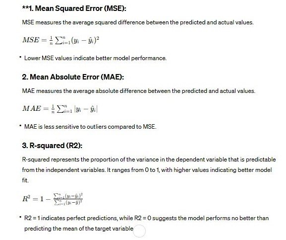
Regression Model Evaluation:

 

4. Residual Analysis:

Residual analysis involves examining the distribution of residuals (the differences between actual and predicted values). Key components include:

• Residual Plot: A scatter plot of residuals against predicted values helps identify patterns or heteroscedasticity.
• Normality Tests: Assessing whether residuals follow a normal distribution using statistical tests.
• Homoscedasticity Tests: Checking for consistent variance in residuals.

5. Cross-Validation:

Similar to classification, cross-validation is valuable for regression models. Techniques like k-fold cross-validation or leave-one-out cross-validation provide a more robust estimate of a model’s generalization performance.

Cross-validation helps prevent overfitting to the training data and provides insights into how the model performs on unseen data.

Common Considerations for Model Evaluation:

1. Overfitting and Underfitting:

• Overfitting: Occurs when a model performs well on the training data but poorly on unseen data. Regularization techniques, cross-validation, and monitoring training/validation performance can help mitigate overfitting.
• Underfitting: Occurs when a model is too simplistic to capture the underlying patterns in the data. Increasing model complexity or using more advanced algorithms may be necessary.

2. Bias-Variance Tradeoff:

• Bias: Error introduced by approximating a real-world problem, leading to the model missing relevant relationships. High bias can result in underfitting.
• Variance: Error introduced by too much complexity, leading to the model being overly sensitive to noise in the training data. High variance can result in overfitting.

Finding an appropriate balance between bias and variance is crucial for model generalization.

3. Hyperparameter Tuning:

Hyperparameter tuning involves adjusting the settings of a model to optimize its performance. Techniques include grid search, random search, and more advanced optimization algorithms.

4. Feature Importance:

Understanding feature importance helps identify which features contribute most to a model’s predictions. Techniques like permutation importance or model-specific feature importance methods (e.g., tree-based models’ feature importance) can be applied.

5. Model Robustness:

Robust models perform well across different subsets of the data and under various conditions. Ensuring a model is robust requires testing its performance on diverse datasets and in scenarios it may encounter in the real world.

Evaluating Survival Analysis models is crucial to assess their performance, reliability, and generalizability. Several metrics and techniques are employed to gauge the effectiveness of these models in predicting the time-to-event outcomes.

The evaluation of survival analysis models involves a combination of quantitative metrics, visualization techniques, and clinical relevance assessments. As the field continues to advance, addressing challenges related to model interpretability, real-world evidence, and patient-centric outcomes will be integral to improving the utility and reliability of survival models in diverse healthcare and research settings.

Common approaches and considerations for evaluating survival analysis models:

1. Concordance Index (C-index):

The concordance index, often referred to as the C-index or C-statistic, is a widely used measure for evaluating the discriminatory power of survival models. It assesses the model’s ability to correctly rank the survival times of pairs of subjects. A C-index of 0.5 indicates random chance, while a value of 1.0 indicates perfect discrimination.

2. Time-Dependent Area Under the Curve (AUC):

Similar to the traditional AUC used in classification tasks, the time-dependent AUC considers the area under the curve over time. It provides a dynamic assessment of a model’s discriminatory power throughout the follow-up period.

3. Integrated Brier Score (IBS):

The Brier score measures the mean squared difference between predicted survival probabilities and actual outcomes. The integrated Brier score extends this concept to evaluate the model’s performance across the entire survival curve, providing a summary measure of calibration and discrimination.

4. Log-Likelihood and Akaike Information Criterion (AIC):

The log-likelihood quantifies how well the model predicts the observed survival times. The AIC takes into account the model’s goodness of fit while penalizing for complexity. Lower AIC values indicate better-fitting models.

5. Calibration Plots:

Calibration plots visually compare predicted survival probabilities against observed outcomes. A well-calibrated model should show points lying close to the 45-degree line, indicating agreement between predicted and observed survival probabilities.

6. Time-Dependent Sensitivity and Specificity:

If the survival model is used for binary classification tasks, sensitivity and specificity can be calculated at different time points to evaluate the model’s performance at specific durations.

7. Decision Curve Analysis (DCA):

DCA assesses the clinical utility of a model by evaluating the net benefit across a range of threshold probabilities. It provides insights into whether the model’s predictions are beneficial for decision-making in a particular clinical context.

8. Recalibration:

Recalibration assesses how well the predicted survival probabilities align with the observed outcomes. It involves dividing the cohort into risk strata and comparing predicted and observed survival within each stratum.

Considerations for Evaluation:

1. Censoring Handling:

Since survival analysis often involves censored data, it’s crucial to evaluate how well the model handles censoring. Metrics and plots should account for the presence of censored observations.

2. Clinical Relevance:

Metrics should be interpreted in the context of the clinical problem. For example, the C-index might be high, but it’s essential to assess whether the improvement in discrimination is clinically meaningful.

3. External Validation:

Models should be validated on external datasets to assess their generalizability. Internal validation, such as bootstrapping or cross-validation, helps estimate the model’s performance on the same dataset it was trained on.

4. Model Assumptions:

Evaluate whether the model assumptions, such as proportional hazards assumption in Cox Regression, hold true. Residual analysis and checks for violations of assumptions are essential.

5. Clinical Interpretability:

Consider the clinical interpretability of the model. Complex models might achieve high performance metrics, but their interpretability and usability in a clinical setting should be evaluated.

6. Robustness:

Assess the robustness of the model to variations in the dataset. Small changes in data or different sampling may affect model performance.

Future Trends in Model Evaluation:

1. Explainability and Transparency:

As models become more complex, there’s an increasing emphasis on developing methods to explain their predictions, especially in medical and clinical contexts where interpretability is crucial.

2. Integration with Real-World Evidence:

The integration of survival models with real-world evidence, such as electronic health records, will become more common for robust validation and evaluation in diverse patient populations.

3. Patient-Centric Outcomes:

Evaluating models based on patient-centric outcomes, such as quality of life, will become more prevalent as the focus shifts toward personalized and patient-centered care.

4. Cross-Domain Model Transferability:

Assessing the transferability of survival models across different domains or populations will be a key consideration, especially in scenarios where data heterogeneity is significant.

5. Dynamic Evaluation Metrics:

Developing metrics that dynamically adapt to changes in the dataset or evolving patient characteristics will be essential for maintaining the relevance and accuracy of survival models over time.