Agile TEST MANAGEMENT: Key Principles

Agile test management is a critical component of Agile development methodologies, ensuring that testing processes align with the principles of agility. It involves adapting test strategies and practices to support iterative development, frequent releases, and collaboration between development and testing teams. Agile test management is guided by principles that emphasize collaboration, adaptability, automation, and a user-centric approach. By embracing these principles, teams can effectively integrate testing into the Agile development lifecycle, ensuring that quality is maintained throughout the process. The iterative and collaborative nature of Agile, coupled with a focus on continuous improvement, allows testing teams to deliver high-quality software in a dynamic and rapidly evolving environment.

Early and Continuous Testing:

  • Principle:

Begin testing activities early in the development process and continue testing throughout the entire Agile lifecycle.

  • Explanation:

Early and continuous testing helps identify defects sooner, reducing the cost of fixing issues and ensuring that quality is built into the product from the start.

Collaboration Between Teams:

  • Principle:

Foster collaboration between development, testing, and other cross-functional teams.

  • Explanation:

Close collaboration ensures that testing is integrated seamlessly into development workflows. Testers actively participate in discussions, share insights, and collaborate with developers to deliver a high-quality product.

Test-Driven Development (TDD):

  • Principle:

Embrace Test-Driven Development as a practice where tests are written before the corresponding code.

  • Explanation:

TDD promotes a focus on requirements and encourages the creation of automated tests. This approach ensures that code meets specifications and remains maintainable over time.

Continuous Integration and Continuous Testing:

  • Principle:

Implement continuous integration and continuous testing practices to automate the build, test, and integration processes.

  • Explanation:

Continuous testing in tandem with continuous integration ensures that changes are validated automatically, providing rapid feedback to developers and maintaining a reliable codebase.

Test Automation:

  • Principle:

Prioritize test automation to increase testing efficiency and support the rapid pace of Agile development.

  • Explanation:

Automated tests help expedite the testing process, provide faster feedback, and allow teams to focus on more complex testing activities. This is essential for achieving Agile goals of speed and frequent releases.

Risk-Based Testing:

  • Principle:

Apply risk-based testing to identify and prioritize test efforts based on the impact and likelihood of potential issues.

  • Explanation:

Prioritizing testing based on risk ensures that efforts are directed towards critical areas, enhancing the effectiveness of testing within time constraints.

Adaptability and Flexibility:

  • Principle:

Be adaptable and flexible in response to changing requirements and priorities.

  • Explanation:

Agile environments are dynamic, and testing processes must be agile as well. The ability to adapt to changing requirements and priorities ensures that testing remains aligned with project goals.

Continuous Improvement:

  • Principle:

Embrace a culture of continuous improvement within the testing process.

  • Explanation:

Regularly review and enhance testing practices based on retrospective feedback. Continuous improvement ensures that the testing process evolves to become more efficient and effective over time.

Shift-Left Testing:

  • Principle:

Shift testing activities left in the development process to catch defects earlier.

  • Explanation:

By moving testing activities closer to the beginning of the development cycle, issues are identified and addressed earlier, reducing the cost of fixing defects and enhancing overall product quality.

Clear Communication:

  • Principle:

Maintain clear and open communication between team members, including testers, developers, and other stakeholders.

  • Explanation:

Effective communication ensures that everyone is on the same page regarding testing objectives, progress, and potential challenges. It fosters collaboration and a shared understanding of quality goals.

Metrics for Continuous Feedback:

  • Principle:

Utilize relevant metrics to provide continuous feedback on the testing process.

  • Explanation:

Metrics such as test coverage, defect density, and test pass rates offer insights into the effectiveness of testing efforts. Continuous feedback helps teams make data-driven decisions for improvement.

User-Centric Testing:

  • Principle:

Prioritize testing from the user’s perspective to ensure that the delivered product meets user expectations.

  • Explanation:

User-centric testing considers the end-user experience and helps uncover issues related to usability, accessibility, and overall satisfaction.

Cross-Functional Skills:

  • Principle:

Encourage cross-functional skills within the testing team to enable versatility and collaboration.

  • Explanation:

Testers with a broad skill set, including domain knowledge, programming skills, and automation expertise, can contribute effectively to various aspects of Agile development.

Regression Testing Automation:

  • Principle:

Automate regression testing to ensure that existing functionality remains intact as new features are added.

  • Explanation:

Regression testing automation supports the continuous delivery of new features without introducing unintended side effects or breaking existing functionality.

Big Data Analytics: A Comprehensive Guide

Big Data Analytics has emerged as a transformative force, reshaping the landscape of decision-making and insights across industries. The dynamic landscape of Big Data Analytics reflects not only the technological prowess of our times but also the profound impact it has on shaping a smarter, more informed future. As we embrace the potential of Big Data Analytics, the journey unfolds with endless possibilities, driving innovation and reshaping the way we understand, interpret, and leverage data for a better tomorrow.

Big Data Analytics continues to redefine how organizations extract value from data. The journey from raw data to actionable insights involves a synergy of technologies, methodologies, and human expertise. As we move forward, the evolution of Big Data Analytics promises even greater advancements, empowering businesses, governments, and individuals with the intelligence to navigate the complexities of our data-driven world.

  • Introduction to Big Data Analytics

Big Data Analytics involves the extraction of meaningful insights from vast and complex datasets. As traditional data processing methods became inadequate, Big Data Analytics emerged to harness the power of massive datasets generated in our interconnected world. It encompasses various techniques, tools, and technologies to analyze, interpret, and visualize data for informed decision-making.

Foundations of Big Data Analytics

  1. Volume, Velocity, Variety, Veracity, and Value (5Vs):

Big Data is characterized by the 5Vs, highlighting the challenges posed by the sheer volume, speed, variety, veracity, and value of data.

  1. Data Processing Frameworks:

Technologies like Apache Hadoop and Apache Spark provide scalable and distributed frameworks for processing large datasets.

  1. Storage Technologies:

Distributed storage solutions like Hadoop Distributed File System (HDFS) and cloud-based storage facilitate the storage of vast amounts of data.

Key Technologies in Big Data Analytics

  1. Apache Hadoop:

An open-source framework for distributed storage and processing of large datasets using a cluster of commodity hardware.

  1. Apache Spark:

A fast and general-purpose cluster-computing framework for large-scale data processing, offering in-memory processing capabilities.

  1. NoSQL Databases:

Non-relational databases like MongoDB and Cassandra accommodate diverse data types and support horizontal scaling.

  1. Machine Learning:

Integration of machine learning algorithms for predictive analytics, pattern recognition, and data classification.

  1. Data Visualization Tools:

Tools like Tableau and Power BI enable the creation of intuitive visual representations for better data interpretation.

Applications of Big Data Analytics

  1. Healthcare Analytics:

Enhancing patient care, predicting disease outbreaks, and optimizing healthcare operations through data-driven insights.

  1. Finance and Banking:

Fraud detection, risk management, and personalized financial services driven by analytics.

  1. Retail and E-Commerce:

Customer behavior analysis, personalized recommendations, and supply chain optimization.

  1. Manufacturing and Industry 4.0:

Predictive maintenance, quality control, and optimization of production processes.

  1. Smart Cities:

Utilizing data for urban planning, traffic management, and resource optimization in city infrastructure.

Challenges in Big Data Analytics

  1. Data Privacy and Security:

Concerns about unauthorized access and misuse of sensitive information.

  1. Data Quality and Integration:

Ensuring the accuracy and integration of diverse datasets for meaningful analysis.

  1. Scalability:

Managing the scalability of infrastructure to handle ever-growing datasets.

  1. Talent Shortage:

The scarcity of skilled professionals well-versed in Big Data Analytics technologies.

Future Trends in Big Data Analytics

  1. Edge Computing:

Analyzing data closer to the source, reducing latency and optimizing bandwidth usage.

  1. Explainable AI:

Enhancing transparency and interpretability in machine learning models.

  1. Automated Machine Learning:

Streamlining the machine learning model development process for broader adoption.

  1. Blockchain Integration:

Ensuring enhanced security and transparency in data transactions.

Top Trends in AI for 2024

Artificial intelligence (AI) is one of the most dynamic and influential fields of technology today. It has the potential to transform various industries, sectors and domains, from healthcare to education, from entertainment to security, from manufacturing to agriculture. As we enter the year 2024, let us take a look at some of the top trends in AI that are expected to shape the future of innovation and society.

  • Explainable AI:

As AI systems become more complex and powerful, there is a growing need for transparency and accountability in how they make decisions and perform actions. Explainable AI (XAI) is a branch of AI that aims to provide human-understandable explanations for the behavior and outcomes of AI models. XAI can help increase trust, confidence and adoption of AI solutions, as well as enable ethical and responsible use of AI.

  • Federated Learning:

Federated learning is a distributed learning paradigm that allows multiple devices or nodes to collaboratively train a shared AI model without exchanging raw data. This can help preserve data privacy and security, as well as reduce communication and computation costs. Federated learning can enable scalable and efficient AI applications in scenarios where data is distributed, sensitive or scarce, such as edge computing, healthcare or finance.

  • Neurosymbolic AI:

Neurosymbolic AI is an emerging approach that combines the strengths of neural networks and symbolic reasoning. Neural networks are good at learning from data and handling uncertainty, but they often lack interpretability and generalization. Symbolic reasoning is good at representing knowledge and logic, but it often requires manual encoding and suffers from brittleness. Neurosymbolic AI can leverage the advantages of both methods to create more robust, versatile and intelligent AI systems.

  • SelfSupervised Learning:

Self-supervised learning is a form of unsupervised learning that uses the data itself as a source of supervision. Instead of relying on external labels or rewards, self-supervised learning generates its own learning objectives or tasks from the data, such as predicting missing words, colors or sounds. Self-supervised learning can help unlock the vast potential of unlabeled data, as well as enable more autonomous and efficient learning for AI models.

  • Artificial General Intelligence:

Artificial general intelligence (AGI) is the ultimate goal of AI research, which is to create machines that can perform any intellectual task that humans can. AGI is still a distant and elusive vision, but there are some promising signs of progress and breakthroughs in this direction. Some of the challenges and opportunities for achieving AGI include creating more human-like cognition, reasoning and emotions, integrating multiple modalities and domains, and aligning AI goals with human values and ethics.

Trends

Advanced Natural Language Processing (NLP):

  • Contextual Understanding:

AI systems are expected to achieve a deeper understanding of context in language, enabling more accurate and context-aware natural language interactions. This involves advancements in semantic understanding and sentiment analysis.

  • Multilingual Capabilities:

Continued progress in multilingual NLP models, allowing AI systems to comprehend and generate content in multiple languages with improved accuracy and fluency.

Generative AI and Creativity:

  • AI-Generated Content:

The rise of AI-generated content across various domains, including art, music, and literature. AI systems are becoming more proficient in creating content that resonates with human preferences and creativity.

  • Enhanced Creativity Tools:

Integration of AI into creative tools for professionals, assisting artists, writers, and musicians in ideation, content creation, and creative exploration.

Explainable AI (XAI):

  • Interpretable Models:

Increased emphasis on creating AI models that are more interpretable and transparent. This trend is essential for building trust in AI systems, especially in critical applications like healthcare and finance.

  • Ethical AI Practices:

Growing awareness and implementation of ethical AI practices, ensuring that AI decisions are explainable, fair, and free from biases.

Edge AI and IoT Integration:

  • On-Device AI:

Continued advancements in on-device AI capabilities, enabling more processing to occur directly on edge devices. This reduces latency, enhances privacy, and optimizes bandwidth usage.

  • AIoT (AI + Internet of Things):

The integration of AI with IoT devices for smarter, more autonomous systems. This includes applications in smart homes, industrial IoT, and healthcare.

AI in Healthcare:

  • Personalized Medicine:

AI-driven approaches for personalized treatment plans, drug discovery, and diagnostics. AI is expected to play a crucial role in tailoring healthcare solutions to individual patient profiles.

  • Health Monitoring:

AI-powered health monitoring systems that leverage wearables and sensors for continuous tracking of health parameters, facilitating early disease detection and prevention.

Autonomous Systems and Robotics:

  • Robotic Process Automation (RPA):

Continued growth in RPA, with more businesses adopting AI-driven automation for routine and repetitive tasks across industries.

  • Autonomous Vehicles:

Advancements in AI algorithms for self-driving cars and other autonomous vehicles, with a focus on safety, efficiency, and real-world adaptability.

AI in Cybersecurity:

  • Threat Detection:

AI-powered cybersecurity solutions that can detect and respond to evolving cyber threats in real-time. This includes the use of machine learning for anomaly detection and behavior analysis.

  • Adversarial AI Defense:

Development of AI systems to counter adversarial attacks, ensuring the robustness and security of AI models against manipulation.

Quantum Computing and AI:

  • Hybrid QuantumAI Systems:

Exploration of synergies between quantum computing and AI for solving complex problems. Quantum computing may offer advantages in optimization tasks and machine learning algorithms.

  • Quantum Machine Learning:

Research and development in quantum machine learning algorithms that leverage the unique properties of quantum systems for enhanced computational power.

AI Governance and Regulation:

  • Ethical AI Guidelines:

Growing efforts to establish global standards and guidelines for ethical AI development and deployment. Governments and industry bodies are likely to play a more active role in regulating AI practices.

  • Responsible AI:

Increased focus on responsible AI practices, emphasizing transparency, accountability, and fairness in AI decision-making processes.

AI Democratization:

  • Accessible AI Tools:

Continued efforts to make AI tools and technologies more accessible to individuals and smaller businesses. This includes the development of user-friendly platforms and AI-as-a-Service offerings.

  • AI Education:

Increased emphasis on AI education and literacy across diverse demographics. Initiatives to empower people with the skills needed to understand, use, and contribute to AI technologies.

Disclaimer: This article is provided for informational purposes only, based on publicly available knowledge. It is not a substitute for professional advice, consultation, or medical treatment. Readers are strongly advised to seek guidance from qualified professionals, advisors, or healthcare practitioners for any specific concerns or conditions. The content on intactone.com is presented as general information and is provided “as is,” without any warranties or guarantees. Users assume all risks associated with its use, and we disclaim any liability for any damages that may occur as a result.

Normal Distribution: Importance, Central Limit Theorem

Normal distribution, or the Gaussian distribution, is a fundamental probability distribution that describes how data values are distributed symmetrically around a mean. Its graph forms a bell-shaped curve, with most data points clustering near the mean and fewer occurring as they deviate further. The curve is defined by two parameters: the mean (μ) and the standard deviation (σ), which determine its center and spread. Normal distribution is widely used in statistics, natural sciences, and social sciences for analysis and inference.

The general form of its probability density function is:

The parameter μ is the mean or expectation of the distribution (and also its median and mode), while the parameter σ is its standard deviation. The variance of the distribution is σ^2. A random variable with a Gaussian distribution is said to be normally distributed, and is called a normal deviate.

Normal distributions are important in statistics and are often used in the natural and social sciences to represent real-valued random variables whose distributions are not known. Their importance is partly due to the central limit theorem. It states that, under some conditions, the average of many samples (observations) of a random variable with finite mean and variance is itself a random variable whose distribution converges to a normal distribution as the number of samples increases. Therefore, physical quantities that are expected to be the sum of many independent processes, such as measurement errors, often have distributions that are nearly normal.

A normal distribution is sometimes informally called a bell curve. However, many other distributions are bell-shaped (such as the Cauchy, Student’s t, and logistic distributions).

Importance of Normal Distribution:

  1. Foundation of Statistical Inference

The normal distribution is central to statistical inference. Many parametric tests, such as t-tests and ANOVA, are based on the assumption that the data follows a normal distribution. This simplifies hypothesis testing, confidence interval estimation, and other analytical procedures.

  1. Real-Life Data Approximation

Many natural phenomena and datasets, such as heights, weights, IQ scores, and measurement errors, tend to follow a normal distribution. This makes it a practical and realistic model for analyzing real-world data, simplifying interpretation and analysis.

  1. Basis for Central Limit Theorem (CLT)

The normal distribution is critical in understanding the Central Limit Theorem, which states that the sampling distribution of the sample mean approaches a normal distribution as the sample size increases, regardless of the population’s actual distribution. This enables statisticians to make predictions and draw conclusions from sample data.

  1. Application in Quality Control

In industries, normal distribution is widely used in quality control and process optimization. Control charts and Six Sigma methodologies assume normality to monitor processes and identify deviations or defects effectively.

  1. Probability Calculations

The normal distribution allows for the easy calculation of probabilities for different scenarios. Its standardized form, the z-score, simplifies these calculations, making it easier to determine how data points relate to the overall distribution.

  1. Modeling Financial and Economic Data

In finance and economics, normal distribution is used to model returns, risks, and forecasts. Although real-world data often exhibit deviations, normal distribution serves as a baseline for constructing more complex models.

Central limit theorem

In probability theory, the central limit theorem (CLT) establishes that, in many situations, when independent random variables are added, their properly normalized sum tends toward a normal distribution (informally a bell curve) even if the original variables themselves are not normally distributed. The theorem is a key concept in probability theory because it implies that probabilistic and statistical methods that work for normal distributions can be applicable to many problems involving other types of distributions. This theorem has seen many changes during the formal development of probability theory. Previous versions of the theorem date back to 1810, but in its modern general form, this fundamental result in probability theory was precisely stated as late as 1920, thereby serving as a bridge between classical and modern probability theory.

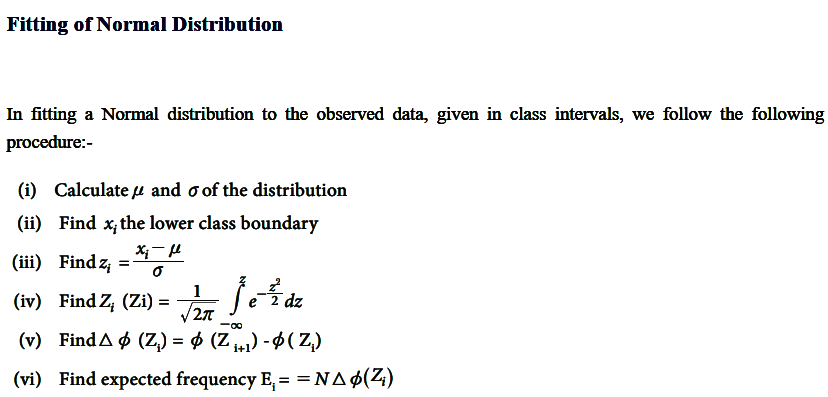
Characteristics Fitting a Normal Distribution

Poisson Distribution: Importance Conditions Constants, Fitting of Poisson Distribution

Poisson distribution is a probability distribution used to model the number of events occurring within a fixed interval of time, space, or other dimensions, given that these events occur independently and at a constant average rate.

Importance

  1. Modeling Rare Events: Used to model the probability of rare events, such as accidents, machine failures, or phone call arrivals.
  2. Applications in Various Fields: Applicable in business, biology, telecommunications, and reliability engineering.
  3. Simplifies Complex Processes: Helps analyze situations with numerous trials and low probability of success per trial.
  4. Foundation for Queuing Theory: Forms the basis for queuing models used in service and manufacturing industries.
  5. Approximation of Binomial Distribution: When the number of trials is large, and the probability of success is small, Poisson distribution approximates the binomial distribution.

Conditions for Poisson Distribution

  1. Independence: Events must occur independently of each other.
  2. Constant Rate: The average rate (λ) of occurrence is constant over time or space.
  3. Non-Simultaneous Events: Two events cannot occur simultaneously within the defined interval.
  4. Fixed Interval: The observation is within a fixed time, space, or other defined intervals.

Constants

  1. Mean (λ): Represents the expected number of events in the interval.
  2. Variance (λ): Equal to the mean, reflecting the distribution’s spread.
  3. Skewness: The distribution is skewed to the right when λ is small and becomes symmetric as λ increases.
  4. Probability Mass Function (PMF): P(X = k) = [e^−λ*λ^k] / k!, Where is the number of occurrences, is the base of the natural logarithm, and λ is the mean.

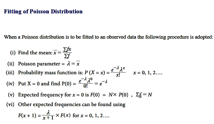
Fitting of Poisson Distribution

When a Poisson distribution is to be fitted to an observed data the following procedure is adopted:

Binomial Distribution: Importance Conditions, Constants

The binomial distribution is a probability distribution that summarizes the likelihood that a value will take one of two independent values under a given set of parameters or assumptions. The underlying assumptions of the binomial distribution are that there is only one outcome for each trial, that each trial has the same probability of success, and that each trial is mutually exclusive, or independent of each other.

In probability theory and statistics, the binomial distribution with parameters n and p is the discrete probability distribution of the number of successes in a sequence of n independent experiments, each asking a yes, no question, and each with its own Boolean-valued outcome: success (with probability p) or failure (with probability q = 1 − p). A single success/failure experiment is also called a Bernoulli trial or Bernoulli experiment, and a sequence of outcomes is called a Bernoulli process; for a single trial, i.e., n = 1, the binomial distribution is a Bernoulli distribution. The binomial distribution is the basis for the popular binomial test of statistical significance.

The binomial distribution is frequently used to model the number of successes in a sample of size n drawn with replacement from a population of size N. If the sampling is carried out without replacement, the draws are not independent and so the resulting distribution is a hypergeometric distribution, not a binomial one. However, for N much larger than n, the binomial distribution remains a good approximation, and is widely used

The binomial distribution is a common discrete distribution used in statistics, as opposed to a continuous distribution, such as the normal distribution. This is because the binomial distribution only counts two states, typically represented as 1 (for a success) or 0 (for a failure) given a number of trials in the data. The binomial distribution, therefore, represents the probability for x successes in n trials, given a success probability p for each trial.

Binomial distribution summarizes the number of trials, or observations when each trial has the same probability of attaining one particular value. The binomial distribution determines the probability of observing a specified number of successful outcomes in a specified number of trials.

The binomial distribution is often used in social science statistics as a building block for models for dichotomous outcome variables, like whether a Republican or Democrat will win an upcoming election or whether an individual will die within a specified period of time, etc.

Importance

For example, adults with allergies might report relief with medication or not, children with a bacterial infection might respond to antibiotic therapy or not, adults who suffer a myocardial infarction might survive the heart attack or not, a medical device such as a coronary stent might be successfully implanted or not. These are just a few examples of applications or processes in which the outcome of interest has two possible values (i.e., it is dichotomous). The two outcomes are often labeled “success” and “failure” with success indicating the presence of the outcome of interest. Note, however, that for many medical and public health questions the outcome or event of interest is the occurrence of disease, which is obviously not really a success. Nevertheless, this terminology is typically used when discussing the binomial distribution model. As a result, whenever using the binomial distribution, we must clearly specify which outcome is the “success” and which is the “failure”.

The binomial distribution model allows us to compute the probability of observing a specified number of “successes” when the process is repeated a specific number of times (e.g., in a set of patients) and the outcome for a given patient is either a success or a failure. We must first introduce some notation which is necessary for the binomial distribution model.

First, we let “n” denote the number of observations or the number of times the process is repeated, and “x” denotes the number of “successes” or events of interest occurring during “n” observations. The probability of “success” or occurrence of the outcome of interest is indicated by “p”.

The binomial equation also uses factorials. In mathematics, the factorial of a non-negative integer k is denoted by k!, which is the product of all positive integers less than or equal to k. For example,

  • 4! = 4 x 3 x 2 x 1 = 24,
  • 2! = 2 x 1 = 2,
  • 1!=1.
  • There is one special case, 0! = 1.

Conditions

  • The number of observations n is fixed.
  • Each observation is independent.
  • Each observation represents one of two outcomes (“success” or “failure”).
  • The probability of “success” p is the same for each outcome

Constants

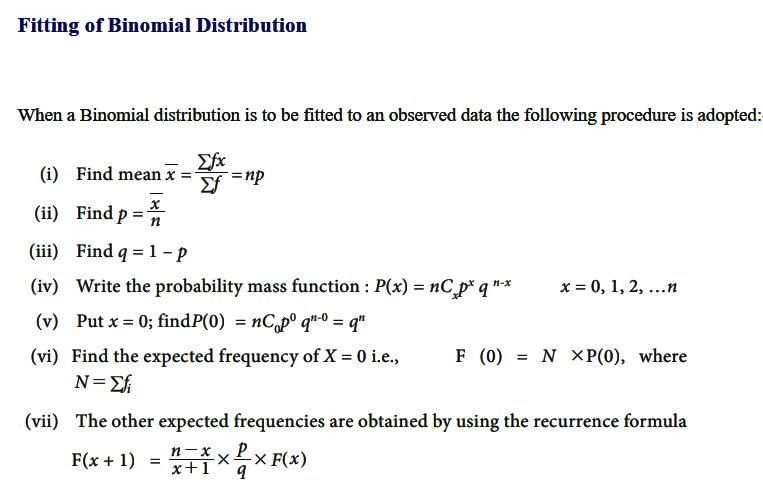
Fitting of Binomial Distribution

Fitting of probability distribution to a series of observed data helps to predict the probability or to forecast the frequency of occurrence of the required variable in a certain desired interval.

To fit any theoretical distribution, one should know its parameters and probability distribution. Parameters of Binomial distribution are n and p. Once p and n are known, binomial probabilities for different random events and the corresponding expected frequencies can be computed. From the given data we can get n by inspection. For binomial distribution, we know that mean is equal to np hence we can estimate p as = mean/n. Thus, with these n and p one can fit the binomial distribution.

There are many probability distributions of which some can be fitted more closely to the observed frequency of the data than others, depending on the characteristics of the variables. Therefore, one needs to select a distribution that suits the data well.

Important Terminologies: Variable, Quantitative Variable, Qualitative Variable, Discrete Variable, Continuous Variable, Dependent Variable, Independent Variable, Frequency, Class Interval, Tally Bar

Important Terminologies:

  • Variable:

Variable is any characteristic, number, or quantity that can be measured or quantified. It can take on different values, which may vary across individuals, objects, or conditions, and is essential in data analysis for observing relationships and patterns.

  • Quantitative Variable:

Quantitative variable is a variable that is measured in numerical terms, such as age, weight, or income. It represents quantities and can be used for mathematical operations, making it suitable for statistical analysis.

  • Qualitative Variable:

Qualitative variable represents categories or attributes, rather than numerical values. Examples include gender, color, or occupation. These variables are non-numeric and are often used in classification and descriptive analysis.

  • Discrete Variable:

Discrete variable is a type of quantitative variable that takes distinct, separate values. These values are countable and cannot take on intermediate values. For example, the number of children in a family is a discrete variable.

  • Continuous Variable:

Continuous variable is a quantitative variable that can take an infinite number of values within a given range. These variables can have decimals or fractions. Examples include height, temperature, or time.

  • Dependent Variable:

Dependent variable is the outcome or response variable that is being measured in an experiment or study. Its value depends on the changes in one or more independent variables. It is the variable of interest in hypothesis testing.

  • Independent Variable:

An independent variable is the variable that is manipulated or controlled in an experiment. It is used to observe its effect on the dependent variable. For example, in a study on plant growth, the amount of water given would be the independent variable.

  • Frequency:

Frequency refers to the number of times a particular value or category occurs in a dataset. It is used in statistical analysis to summarize the distribution of data points within various categories or intervals.

  • Class Interval:

A class interval is a range of values within which data points fall in grouped data. It is commonly used in frequency distributions to organize data into specific ranges, such as “0-10,” “11-20,” etc.

  • Tally Bar:

A tally bar is a method of recording data frequency by using vertical lines. Every group of five tallies (four vertical lines and a fifth diagonal line) represents five occurrences, helping to visually track counts in surveys or experiments.

Important Terminologies in Statistics: Data, Raw Data, Primary Data, Secondary Data, Population, Census, Survey, Sample Survey, Sampling, Parameter, Unit, Variable, Attribute, Frequency, Seriation, Individual, Discrete and Continuous

Statistics is the branch of mathematics that involves the collection, analysis, interpretation, presentation, and organization of data. It helps in drawing conclusions and making decisions based on data patterns, trends, and relationships. Statistics uses various methods such as probability theory, sampling, and hypothesis testing to summarize data and make predictions. It is widely applied across fields like economics, medicine, social sciences, business, and engineering to inform decisions and solve real-world problems.

1. Data

Data is information collected for analysis, interpretation, and decision-making. It can be qualitative (descriptive, such as color or opinions) or quantitative (numerical, such as age or income). Data serves as the foundation for statistical studies, enabling insights into patterns, trends, and relationships.

2. Raw Data

Raw data refers to unprocessed or unorganized information collected from observations or experiments. It is the initial form of data, often messy and requiring cleaning or sorting for meaningful analysis. Examples include survey responses or experimental results.

3. Primary Data

Primary data is original information collected directly by a researcher for a specific purpose. It is firsthand and authentic, obtained through methods like surveys, experiments, or interviews. Primary data ensures accuracy and relevance to the study but can be time-consuming to collect.

4. Secondary Data

Secondary data is pre-collected information used by researchers for analysis. It includes published reports, government statistics, and historical data. Secondary data saves time and resources but may lack relevance or accuracy for specific studies compared to primary data.

5. Population

A population is the entire group of individuals, items, or events that share a common characteristic and are the subject of a study. It includes every possible observation or unit, such as all students in a school or citizens in a country.

6. Census

A census involves collecting data from every individual or unit in a population. It provides comprehensive and accurate information but requires significant resources and time. Examples include national population censuses conducted by governments.

7. Survey

A survey gathers information from respondents using structured tools like questionnaires or interviews. It helps collect opinions, behaviors, or characteristics. Surveys are versatile and widely used in research, marketing, and public policy analysis.

8. Sample Survey

A sample survey collects data from a representative subset of the population. It saves time and costs while providing insights that can generalize to the entire population, provided the sampling method is unbiased and rigorous.

9. Sampling

Sampling is the process of selecting a portion of the population for study. It ensures efficiency and feasibility in data collection. Sampling methods include random, stratified, and cluster sampling, each suited to different study designs.

10. Parameter

A parameter is a measurable characteristic that describes a population, such as the mean, median, or standard deviation. Unlike a statistic, which pertains to a sample, a parameter is specific to the entire population.

11. Unit

A unit is an individual entity in a population or sample being studied. It can represent a person, object, transaction, or observation. Each unit contributes to the dataset, forming the basis for analysis.

12. Variable

A variable is a characteristic or property that can change among individuals or items. It can be quantitative (e.g., age, weight) or qualitative (e.g., color, gender). Variables are the focus of statistical analysis to study relationships and trends.

13. Attribute

An attribute is a qualitative feature that describes a characteristic of a unit. Attributes are non-measurable but observable, such as eye color, marital status, or type of vehicle.

14. Frequency

Frequency represents how often a specific value or category appears in a dataset. It is key in descriptive statistics, helping to summarize and visualize data patterns through tables, histograms, or frequency distributions.

15. Seriation

Seriation is the arrangement of data in sequential or logical order, such as ascending or descending by size, date, or importance. It aids in identifying patterns and organizing datasets for analysis.

16. Individual

An individual is a single member or unit of the population or sample being analyzed. It is the smallest element for data collection and analysis, such as a person in a demographic study or a product in a sales dataset.

17. Discrete Variable

A discrete variable takes specific, separate values, often integers. It is countable and cannot assume fractional values, such as the number of employees in a company or defective items in a batch.

18. Continuous Variable

A continuous variable can take any value within a range and represents measurable quantities. Examples include temperature, height, and time. Continuous variables are essential for analyzing trends and relationships in datasets.

Perquisites of Good Classification of Data

Good classification of data is essential for organizing, analyzing, and interpreting the data effectively. Proper classification helps in understanding the structure and relationships within the data, enabling informed decision-making.

1. Clear Objective

Good classification should have a clear objective, ensuring that the classification scheme serves a specific purpose. It should be aligned with the goal of the study, whether it’s identifying trends, comparing categories, or finding patterns in the data. This helps in determining which variables or categories should be included and how they should be grouped.

2. Homogeneity within Classes

Each class or category within the classification should contain items or data points that are similar to each other. This homogeneity within the classes allows for better analysis and comparison. For example, when classifying people by age, individuals within a particular age group should share certain characteristics related to that age range, ensuring that each class is internally consistent.

3. Heterogeneity between Classes

While homogeneity is crucial within classes, there should be noticeable differences between the various classes. A good classification scheme should maximize the differences between categories, ensuring that each group represents a distinct set of data. This helps in making meaningful distinctions and drawing useful comparisons between groups.

4. Exhaustiveness

Good classification system must be exhaustive, meaning that it should cover all possible data points in the dataset. There should be no omission, and every item must fit into one and only one class. Exhaustiveness ensures that the classification scheme provides a complete understanding of the dataset without leaving any data unclassified.

5. Mutually Exclusive

Classes should be mutually exclusive, meaning that each data point can belong to only one class. This avoids ambiguity and ensures clarity in analysis. For example, if individuals are classified by age group, someone who is 25 years old should only belong to one age class (such as 20-30 years), preventing overlap and confusion.

6. Simplicity

Good classification should be simple and easy to understand. The classification categories should be well-defined and not overly complicated. Simplicity ensures that the classification scheme is accessible and can be easily used for analysis by various stakeholders, from researchers to policymakers. Overly complex classification schemes may lead to confusion and errors.

7. Flexibility

Good classification system should be flexible enough to accommodate new data or changing circumstances. As new categories or data points emerge, the classification scheme should be adaptable without requiring a complete overhaul. Flexibility allows the classification to remain relevant and useful over time, particularly in dynamic fields like business or technology.

8. Consistency

Consistency in classification is essential for maintaining reliability in data analysis. A good classification system ensures that the same criteria are applied uniformly across all classes. For example, if geographical regions are being classified, the same boundaries and criteria should be consistently applied to avoid confusion or inconsistency in reporting.

9. Appropriateness

Good classification should be appropriate for the type of data being analyzed. The classification scheme should fit the nature of the data and the specific objectives of the analysis. Whether classifying data by geographical location, age, or income, the scheme should be meaningful and suited to the research question, ensuring that it provides valuable insights.

Quantitative and Qualitative Classification of Data

Data refers to raw, unprocessed facts and figures that are collected for analysis and interpretation. It can be qualitative (descriptive, like colors or opinions) or quantitative (numerical, like age or sales figures). Data is the foundation of statistics and research, providing the basis for drawing conclusions, making decisions, and discovering patterns or trends. It can come from various sources such as surveys, experiments, or observations. Proper organization and analysis of data are crucial for extracting meaningful insights and informing decisions across various fields.

Quantitative Classification of Data:

Quantitative classification of data involves grouping data based on numerical values or measurable quantities. It is used to organize continuous or discrete data into distinct classes or intervals to facilitate analysis. The data can be categorized using methods such as frequency distributions, where values are grouped into ranges (e.g., 0-10, 11-20) or by specific numerical characteristics like age, income, or height. This classification helps in summarizing large datasets, identifying patterns, and conducting statistical analysis such as finding the mean, median, or mode. It enables clearer insights and easier comparisons of quantitative data across different categories.

Features of Quantitative Classification of Data:

  • Based on Numerical Data

Quantitative classification specifically deals with numerical data, such as measurements, counts, or any variable that can be expressed in numbers. Unlike qualitative data, which deals with categories or attributes, quantitative classification groups data based on values like height, weight, income, or age. This classification method is useful for data that can be measured and involves identifying patterns in numerical values across different ranges.

  • Division into Classes or Intervals

In quantitative classification, data is often grouped into classes or intervals to make analysis easier. These intervals help in summarizing a large set of data and enable quick comparisons. For example, when classifying income levels, data can be grouped into intervals such as “0-10,000,” “10,001-20,000,” etc. The goal is to reduce the complexity of individual data points by organizing them into manageable segments, making it easier to observe trends and patterns.

  • Class Limits

Each class in a quantitative classification has defined class limits, which represent the range of values that belong to that class. For example, in the case of age, a class may be defined with the limits 20-30, where the class includes all data points between 20 and 30 (inclusive). The lower and upper limits are crucial for ensuring that data is classified consistently and correctly into appropriate ranges.

  • Frequency Distribution

Frequency distribution is a key feature of quantitative classification. It refers to how often each class or interval appears in a dataset. By organizing data into classes and counting the number of occurrences in each class, frequency distributions provide insights into the spread of the data. This helps in identifying which ranges or intervals contain the highest concentration of values, allowing for more targeted analysis.

  • Continuous and Discrete Data

Quantitative classification can be applied to both continuous and discrete data. Continuous data, like height or temperature, can take any value within a range and is often classified into intervals. Discrete data, such as the number of people in a group or items sold, involves distinct, countable values. Both types of quantitative data are classified differently, but the underlying principle of grouping into classes remains the same.

  • Use of Central Tendency Measures

Quantitative classification often involves calculating measures of central tendency, such as the mean, median, and mode, for each class or interval. These measures provide insights into the typical or average values within each class. For example, by calculating the average income within specific income brackets, researchers can better understand the distribution of income across the population.

  • Graphical Representation

Quantitative classification is often complemented by graphical tools such as histograms, bar charts, and frequency polygons. These visual representations provide a clear view of how data is distributed across different classes or intervals, making it easier to detect trends, outliers, and patterns. Graphs also help in comparing the frequencies of different intervals, enhancing the understanding of the dataset.

Qualitative Classification of Data:

Qualitative classification of data involves grouping data based on non-numerical characteristics or attributes. This classification is used for categorical data, where the values represent categories or qualities rather than measurable quantities. Examples include classifying individuals by gender, occupation, marital status, or color. The data is typically organized into distinct groups or classes without any inherent order or ranking. Qualitative classification allows researchers to analyze patterns, relationships, and distributions within different categories, making it easier to draw comparisons and identify trends. It is often used in fields such as social sciences, marketing, and psychology for descriptive analysis.

Features of  Qualitative Classification of Data:

  • Based on Categories or Attributes

Qualitative classification deals with data that is based on categories or attributes, such as gender, occupation, religion, or color. Unlike quantitative data, which is measured in numerical values, qualitative data involves sorting or grouping items into distinct categories based on shared qualities or characteristics. This type of classification is essential for analyzing data that does not have a numerical relationship.

  • No Specific Order or Ranking

In qualitative classification, the categories do not have a specific order or ranking. For instance, when classifying individuals by their profession (e.g., teacher, doctor, engineer), the categories do not imply any hierarchy or ranking order. The lack of a natural sequence or order distinguishes qualitative classification from ordinal data, which involves categories with inherent ranking (e.g., low, medium, high). The focus is on grouping items based on their similarity in attributes.

  • Mutual Exclusivity

Each data point in qualitative classification must belong to one and only one category, ensuring mutual exclusivity. For example, an individual cannot simultaneously belong to both “Male” and “Female” categories in a gender classification scheme. This feature helps to avoid overlap and ambiguity in the classification process. Ensuring mutual exclusivity is crucial for clear analysis and accurate data interpretation.

  • Exhaustiveness

Qualitative classification should be exhaustive, meaning that all possible categories are covered. Every data point should fit into one of the predefined categories. For instance, if classifying by marital status, categories like “Single,” “Married,” “Divorced,” and “Widowed” must encompass all possible marital statuses within the dataset. Exhaustiveness ensures no data is left unclassified, making the analysis complete and comprehensive.

  • Simplicity and Clarity

A good qualitative classification should be simple, clear, and easy to understand. The categories should be well-defined, and the criteria for grouping data should be straightforward. Complexity and ambiguity in categorization can lead to confusion, misinterpretation, or errors in analysis. Simple and clear classification schemes make the data more accessible and improve the quality of research and reporting.

  • Flexibility

Qualitative classification is flexible and can be adapted as new categories or attributes emerge. For example, in a study of professions, new job titles or fields may develop over time, and the classification system can be updated to include these new categories. Flexibility in qualitative classification allows researchers to keep the data relevant and reflective of changes in society, industry, or other fields of interest.

  • Focus on Descriptive Analysis

Qualitative classification primarily focuses on descriptive analysis, which involves summarizing and organizing data into meaningful categories. It is used to explore patterns and relationships within the data, often through qualitative techniques such as thematic analysis or content analysis. The goal is to gain insights into the characteristics or behaviors of individuals, groups, or phenomena rather than making quantitative comparisons.

error: Content is protected !!