Binomial Distribution: Importance Conditions, Constants

The binomial distribution is a probability distribution that summarizes the likelihood that a value will take one of two independent values under a given set of parameters or assumptions. The underlying assumptions of the binomial distribution are that there is only one outcome for each trial, that each trial has the same probability of success, and that each trial is mutually exclusive, or independent of each other.

In probability theory and statistics, the binomial distribution with parameters n and p is the discrete probability distribution of the number of successes in a sequence of n independent experiments, each asking a yes, no question, and each with its own Boolean-valued outcome: success (with probability p) or failure (with probability q = 1 − p). A single success/failure experiment is also called a Bernoulli trial or Bernoulli experiment, and a sequence of outcomes is called a Bernoulli process; for a single trial, i.e., n = 1, the binomial distribution is a Bernoulli distribution. The binomial distribution is the basis for the popular binomial test of statistical significance.

The binomial distribution is frequently used to model the number of successes in a sample of size n drawn with replacement from a population of size N. If the sampling is carried out without replacement, the draws are not independent and so the resulting distribution is a hypergeometric distribution, not a binomial one. However, for N much larger than n, the binomial distribution remains a good approximation, and is widely used

The binomial distribution is a common discrete distribution used in statistics, as opposed to a continuous distribution, such as the normal distribution. This is because the binomial distribution only counts two states, typically represented as 1 (for a success) or 0 (for a failure) given a number of trials in the data. The binomial distribution, therefore, represents the probability for x successes in n trials, given a success probability p for each trial.

Binomial distribution summarizes the number of trials, or observations when each trial has the same probability of attaining one particular value. The binomial distribution determines the probability of observing a specified number of successful outcomes in a specified number of trials.

The binomial distribution is often used in social science statistics as a building block for models for dichotomous outcome variables, like whether a Republican or Democrat will win an upcoming election or whether an individual will die within a specified period of time, etc.

Importance

For example, adults with allergies might report relief with medication or not, children with a bacterial infection might respond to antibiotic therapy or not, adults who suffer a myocardial infarction might survive the heart attack or not, a medical device such as a coronary stent might be successfully implanted or not. These are just a few examples of applications or processes in which the outcome of interest has two possible values (i.e., it is dichotomous). The two outcomes are often labeled “success” and “failure” with success indicating the presence of the outcome of interest. Note, however, that for many medical and public health questions the outcome or event of interest is the occurrence of disease, which is obviously not really a success. Nevertheless, this terminology is typically used when discussing the binomial distribution model. As a result, whenever using the binomial distribution, we must clearly specify which outcome is the “success” and which is the “failure”.

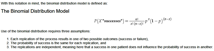
The binomial distribution model allows us to compute the probability of observing a specified number of “successes” when the process is repeated a specific number of times (e.g., in a set of patients) and the outcome for a given patient is either a success or a failure. We must first introduce some notation which is necessary for the binomial distribution model.

First, we let “n” denote the number of observations or the number of times the process is repeated, and “x” denotes the number of “successes” or events of interest occurring during “n” observations. The probability of “success” or occurrence of the outcome of interest is indicated by “p”.

The binomial equation also uses factorials. In mathematics, the factorial of a non-negative integer k is denoted by k!, which is the product of all positive integers less than or equal to k. For example,

  • 4! = 4 x 3 x 2 x 1 = 24,
  • 2! = 2 x 1 = 2,
  • 1!=1.
  • There is one special case, 0! = 1.

Conditions

  • The number of observations n is fixed.
  • Each observation is independent.
  • Each observation represents one of two outcomes (“success” or “failure”).
  • The probability of “success” p is the same for each outcome

Constants

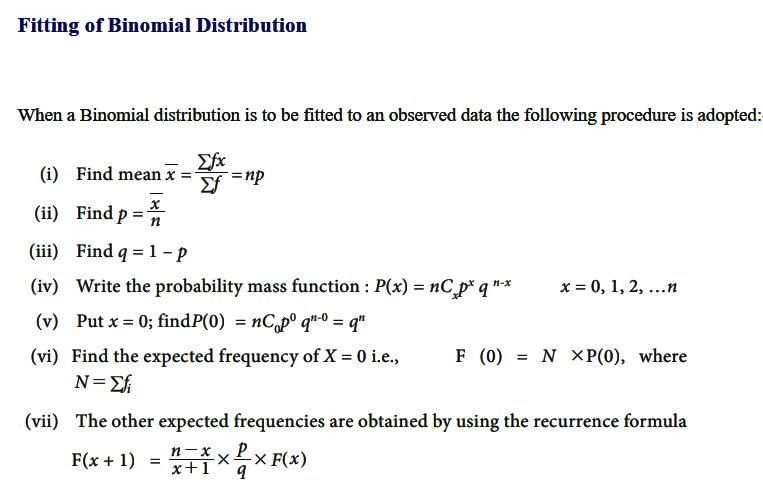
Fitting of Binomial Distribution

Fitting of probability distribution to a series of observed data helps to predict the probability or to forecast the frequency of occurrence of the required variable in a certain desired interval.

To fit any theoretical distribution, one should know its parameters and probability distribution. Parameters of Binomial distribution are n and p. Once p and n are known, binomial probabilities for different random events and the corresponding expected frequencies can be computed. From the given data we can get n by inspection. For binomial distribution, we know that mean is equal to np hence we can estimate p as = mean/n. Thus, with these n and p one can fit the binomial distribution.

There are many probability distributions of which some can be fitted more closely to the observed frequency of the data than others, depending on the characteristics of the variables. Therefore, one needs to select a distribution that suits the data well.

Permutation, Combination

Permutation

In mathematics, a permutation of a set is, loosely speaking, an arrangement of its members into a sequence or linear order, or if the set is already ordered, a rearrangement of its elements. The word “permutation” also refers to the act or process of changing the linear order of an ordered set.

Permutations differ from combinations, which are selections of some members of a set regardless of order. For example, written as tuples, there are six permutations of the set {1,2,3}, namely: (1,2,3), (1,3,2), (2,1,3), (2,3,1), (3,1,2), and (3,2,1). These are all the possible orderings of this three-element set. Anagrams of words whose letters are different are also permutations: the letters are already ordered in the original word, and the anagram is a reordering of the letters. The study of permutations of finite sets is an important topic in the fields of combinatorics and group theory.

Permutations are used in almost every branch of mathematics, and in many other fields of science. In computer science, they are used for analyzing sorting algorithms; in quantum physics, for describing states of particles; and in biology, for describing RNA sequences.

The number of permutations of n distinct objects is n factorial, usually written as n!, which means the product of all positive integers less than or equal to n.

Technically, a permutation of a set S is defined as a bijection from S to itself. That is, it is a function from S to S for which every element occurs exactly once as an image value. This is related to the rearrangement of the elements of S in which each element s is replaced by the corresponding f(s). For example, the permutation (3,1,2) mentioned above is described by the function alpha defined as:

α (1) = 3,

α (2) = 1

α (3) = 2

The collection of all permutations of a set form a group called the symmetric group of the set. The group operation is the composition (performing two given rearrangements in succession), which results in another rearrangement. As properties of permutations do not depend on the nature of the set elements, it is often the permutations of the set {1,2,…n} that are considered for studying permutations.

In elementary combinatorics, the k-permutations, or partial permutations, are the ordered arrangements of k distinct elements selected from a set. When k is equal to the size of the set, these are the permutations of the set.

Combination

A combination is a mathematical technique that determines the number of possible arrangements in a collection of items where the order of the selection does not matter. In combinations, you can select the items in any order.

Combinations can be confused with permutations. However, in permutations, the order of the selected items is essential. For example, the arrangements ab and ba are equal in combinations (considered as one arrangement), while in permutations, the arrangements are different.

Combinations are studied in combinatorics but are also used in different disciplines, including mathematics and finance.

Basics of Set Theory

Set theory, branch of mathematics that deals with the properties of well-defined collections of objects, which may or may not be of a mathematical nature, such as numbers or functions. The theory is less valuable in direct application to ordinary experience than as a basis for precise and adaptable terminology for the definition of complex and sophisticated mathematical concepts.

Fundamental set concepts

In naive set theory, a set is a collection of objects (called members or elements) that is regarded as being a single object. To indicate that an object x is a member of a set A one writes x ∊ A, while x ∉ A indicates that x is not a member of A. A set may be defined by a membership rule (formula) or by listing its members within braces. For example, the set given by the rule “prime numbers less than 10” can also be given by {2, 3, 5, 7}. In principle, any finite set can be defined by an explicit list of its members, but specifying infinite sets requires a rule or pattern to indicate membership; for example, the ellipsis in {0, 1, 2, 3, 4, 5, 6, 7, …} indicates that the list of natural numbers ℕ goes on forever. The empty (or void, or null) set, symbolized by {} or Ø, contains no elements at all. Nonetheless, it has the status of being a set.

A set A is called a subset of a set B (symbolized by A ⊆ B) if all the members of A are also members of B. For example, any set is a subset of itself, and Ø is a subset of any set. If both A ⊆ B and B ⊆ A, then A and B have exactly the same members. Part of the set concept is that in this case A = B; that is, A and B are the same set.

Representation of Sets

Sets can be represented in two ways:

  • Roster Form or Tabular form
  • Set Builder Form

Roster Form

In roster form, all the elements of the set are listed, separated by commas and enclosed between curly braces { }.

Example: If set represents all the leap years between the year 1995 and 2015, then it would be described using Roster form as:

A = {1996,2000,2004,2008,2012}

Also, multiplicity is ignored while representing the sets. e.g. If L represents a set that contains all the letters in the word ADDRESS, the proper Roster form representation would be

L = {A, D, R, E, S }= {S,E,D,A,R} 

L≠ {A, D, D, R, E, S, S}

Set Builder Form

In set builder form, all the elements have a common property. This property is not applicable to the objects that do not belong to the set.

Example: If set S has all the elements which are even prime numbers, it is represented as:

S= { x: x is an even prime number}

where ‘x’ is a symbolic representation that is used to describe the element.

‘:’ means ‘such that’

‘{}’ means ‘the set of all’

So, S = { x:x is an even prime number } is read as ‘the set of all x such that x is an even prime number’. The roster form for this set S would be S = 2. This set contains only one element. Such sets are called singleton/unit sets.

Event: Mutually Exclusive Events, Collectively Exhaustive Events, Independent Events, Simple and Compound Events

Mutually Exclusive Events

When two events (call them “A” and “B”) are Mutually Exclusive it is impossible for them to happen together:

P(A and B) = 0

“The probability of A and B together equals 0 (impossible)”

But, for Mutually Exclusive events, the probability of A or B is the sum of the individual probabilities:

P(A or B) = P(A) + P(B)

“The probability of A or B equals the probability of A plus the probability of B”

Collectively Exhaustive Events

In probability, a set of events is collectively exhaustive if they cover all of the probability space: i.e., the probability of any one of them happening is 100%. If a set of statements is collectively exhaustive, we know at least one of them is true.

If you are rolling a six-sided die, the set of events {1, 2, 3, 4, 5, 6} is collectively exhaustive. Any roll must be represented by one of the set.

Sometimes a small change can make a set that is not collectively exhaustive into one that is. A random integer generated by a computer may be greater than or less than 5, but those are not collectively exhaustive options. Changing one option to “greater than or equal to five” or adding five as an option makes the set fit our criteria.

Another way to describe collectively exhaustive events is that their union must cover all the events within the entire sample space. For example, events A and B are said to be collectively exhaustive if

A U B=S

where S is the sample space.

Independent Events

Independent Events are not affected by previous events.

A coin does not “know” it came up heads before.

And each toss of a coin is a perfect isolated thing.

Probability of an event happening = Number of ways it can happen / Total number of outcomes

Simple and Compound Events

A simple event is one that can only happen in one way in other words, it has a single outcome. If we consider our previous example of tossing a coin: we get one outcome that is a head or a tail.

A compound event is more complex than a simple event, as it involves the probability of more than one outcome. Another way to view compound events is as a combination of two or more simple events.

Simple Event

An event that has a single point of the sample space is known as a simple event in probability.

Probability of an event occurring = No. of favorable outcomes / Total no. of outcomes

Compound Event

If an event has more than one sample point, it is termed as a compound event. The compound events are a little more complex than simple events. These events involve the probability of more than one event occurring together. The total probability of all the outcomes of a compound event is equal to 1.

To calculate probability, the following formula is used:

Probability of an event = [The number of favorable outcomes] / [the number of total outcomes].

First, we find the probability of each event occurring. Then we will multiply these probabilities together. In the case of a compound event, the numerator (number of favourable outcomes) will be greater than 1.

For example, the probability of rolling an odd number on a die, then tossing a head on a coin.

Here P(odd number) = 3/6

P(head) = 1/2

Hence required probability = (3/6)(½ )

= 3/12           

Deseasonalisation of Data

Seasonality is a characteristic of a time series in which the data experiences regular and predictable changes that recur every calendar year. Any predictable fluctuation or pattern that recurs or repeats over a one-year period is said to be seasonal.

Seasonal effects are different from cyclical effects, as seasonal cycles are observed within one calendar year, while cyclical effects, such as boosted sales due to low unemployment rates, can span time periods shorter or longer than one calendar year.

Seasonality Types

There are three common seasonality types: yearly, monthly and weekly.

(i) Yearly seasonality

Yearly seasonality encompasses predictable changes in demand month over month and are consistent on an annual basis. For example, the purchase of swimsuits and sunscreen prior to the summer months and notebooks and pens leading up to the new school year.

(ii) Monthly seasonality

Monthly seasonality covers variations in demand over the course of a month, like the purchasing of items biweekly when paychecks come in or at the end of the month when there’s extra money in the budget.

(iii) Weekly seasonality

Weekly seasonality is a characteristic of more general product consumption and reflects a host of variables. You may find that consumers buy more (or less) of different products on different days of the week.

Challenges in estimating seasonality indices

The seasonality model illustrated here above is a rather naive approach that work for long smooth seasonal time-series. Yet, there are multiple practical difficulties when estimating seasonality:

  • Time-series are short. The lifespan of most consumer goods do not exceed 3 or 4 years. As a result, for a given product, sales history offers on average very few points in the past to estimate each seasonal index (that is to say the values of S(t) during the course of the year, cf. the previous section).
  • Time-series are noisy. Random market fluctuations impact the sales, and make the seasonality more difficult to isolate.
  • Multiple seasonalities are involved. When looking at sales at the store level, the seasonality of the product itself is typically entangled with the seasonality of the store.
  • Other patterns such as trend or product lifecycle also impact time-series, introducing various sort of bias in the estimation.

In many cases, seasonal patterns are removed from time-series data when they’re released on public databases. Data that has been stripped of its seasonal patterns is referred to as seasonally adjusted or deseasonalized data.

Semi Average Method

Under this method, as the name itself suggests semiaverages are calculated to find out the trend values. By semi-averages is meant the averages of the two halves of a series. In this method, thus, the given series is divided into two equal parts (halves) and the arithmetic mean of the values of each part (half) is calculated. The computed means are termed as semi-averages. Each semi-average is paired with the centre of time period of its part. The two pairs are then plotted on a graph paper and the points are joined by a straight line to get the trend. It should be noted that if the data is for even number of years, it can be easily divided into two halves. But if it is for odd number of years, we leave the middle year of the time series and two halves constitute the periods on each side of the middle year.

Advantages:

  1. It is simple method of measuring trend.
  2. It is an objective method because anyone applying this to a given data would get identical trend value.

Disadvantages:

  1. This method can give only linear trend of the data irrespective of whether it exists or not.
  2. This is only a crude method of measuring trend, since we do not know whether the effects of other components are completely eliminated or not.


Uses and Limitations of Time Series

Understanding data

Another benefit of time series analysis is that it can help an analyst to better understand a data set. This is because of the models used in time series analysis help to interpret the true meaning of the data, as touched on previously.

Opportunity to Clean data

The first benefit of time series analysis is that it can help to clean data. This makes it possible to find the true “signal” in a data set, by filtering out the noise. This can mean removing outliers, or applying various averages so as to gain an overall perspective of the meaning of the data.

Of course, cleaning data is a prominent part of almost any kind of data analysis. The true benefit of time series analysis is that it is accomplished with little extra effort.

Forecasting data

Last but not least, a major benefit of time series analysis is that it can be the basis to forecast data. This is because time series analysis by its very nature uncovers patterns in data, which can then be used to predict future data points.

For example, autocorrelation patterns and seasonality measures can be used to predict when a certain data point can be expected. Further, stationarity measures can be used to estimate what the value of that data point will be.

Really, it’s the forecasting aspect of time series analysis that makes it so popular in business applications. Analyzing and understanding past data is all good and well, but it’s being able to predict the future that helps to make optimal business decisions.

Time Series Analysis Helps You Identify Patterns

Memories are fragile and prone to error. You may think that your sales peak before Christmas and hit their bottom in February… but do they really?

The simplest and, in most cases, the most effective form of time series analysis is to simply plot the data on a line chart. With this step, there will no longer be any doubts as to whether or not sales truly peak before Christmas and dip in February.

Limitations

Time series methods draw on vastly different areas in statistics, and lately, machine learning. You have to know a lot about all of these things, in general, to make sense of what you’re doing. There is no real unification of the theory, either.

Often there are ways around getting a model that is time-series based where the predictions are almost as good and is faster to implement. Note that this may or may not blow up in your face later on. In some cases, however, temporal effects are so weak that it makes more sense to just use the non-temporal ones… which can be difficult to explain (the need to check) to a manager if we’ve had to spend 2.5 weeks setting up the tests for temporal effects. Personal experience here.

This is hard stuff, and if you’re not motivated by challenge, you can get overwhelmed. Also, there is, in some other areas of data science, the notion that all we use are ARIMA models and EWMA; while we do often use these tools, we also use RNN and LTSM networks and a whole lot of interesting things.

Most machine learning algorithms don’t deal with time well.

Problems in the Construction of Index Numbers

  1. Difficulties in the Selection of Commodities:

The selection of representative commodities for the index number is another difficulty. The choice of representative commodities is not an easy matter. They have to be selected from a wide range of commodities which the majority of people consume. Again, what were representative commodities some ten years ago may not be representative today. The consumption pattern of consumers might change and thereby make the index number useless. So, the choice of representative commodities presents real difficulties.

  1. Difficulties in the Selection of the Base Period:

The first difficulty relates to the selection of the base year. The base year should be normal. But it is difficult to determine a truly normal year. Moreover, what may be the normal year today may become an abnormal year after some period. Therefore, it is not advisable to have the same year as the base period for a number of years. Rather, it should be changed after ten years or so. But there is no fixed rule for this.

  1. Difficulties in the Collection of Prices:

Another difficulty is that of collecting adequate and accurate prices. It is often not possible to get them from the same source or place. Further, the problem of choice between wholesale and retail prices arises. There are much variations in the retail prices. Therefore, index numbers are based on wholesale prices.

  1. Arbitrary Assigning of Weights:

In calculating weighted price index, a number of difficulties arise. The problem is to give different weights to commodities. The selection of higher weight for one commodity and a lower weight for another is simply arbitrary. There is no set rule and it entirely depends on the investigator. Moreover, the same commodity may have different importance for different consumers. The importance of commodities also changes with the change in the tastes and incomes of consumers and also with the passage of time. Therefore, weights are to be revised from time to time and not fixed arbitrarily.

  1. Not All Purpose:

An index number constructed for a particular purpose cannot be used for some other purpose. For instance, a cost of living index number for industrial workers cannot be used to measure the cost of living of agricultural workers. Thus there are no all purpose index numbers.

  1. International Comparisons not Possible:

International price comparisons are not possible with index numbers. The commodities consumed and included in the construction of an index number differ from country to country. For instance, meat, eggs, cars, and electrical appliance are included in the price index of advanced countries whereas they are not included in that of backward countries. Similarly, weights assigned to commodities are also different. Thus, international comparisons of index numbers are not possible.

  1. Comparisons of Different Places not Possible:

Even if different places within a country are taken, it is not possible to apply the same index number to them. This is because of differences in the consumption habits of people. People living in the northern region consume different commodities than those consumed by the people in the south of India. It is, therefore, not right to apply the same index number to both.

  1. Not Applicable to an Individual:

An index number is not applicable to an individual belonging to a group for which it is constructed. If an index number shows a rise in the price level, an individual may not be affected by it. This is because an index number reflects averages.

  1. Difficulty of Selecting the Method of Averaging:

Another difficulty is to select an appropriate method of calculating averages. There are a number of methods which can be used for this purpose. But all methods give different results from one another. It is, therefore, difficult to decide which method to choose.

  1. Difficulties Arising from Changes Overtime:

In the present times, changes in the nature of commodities are taking place continuously overtime due to technological changes. As a result, new commodities are introduced and people start consuming them in place of the old ones. Moreover, prices of commodities might also change with technical changes. They may fall. But new commodities are not entered into the list of commodities in preparing the index numbers. This makes the index numbers based on old commodities unreal.

Using Regression Lines for Prediction

Linear regression analysis is a powerful technique used for predicting the unknown value of a variable from the known value of another variable.

More precisely, if X and Y are two related variables, then linear regression analysis helps us to predict the value of Y for a given value of X or vice verse.

Using regression to make predictions doesn’t necessarily involve predicting the future. Instead, you predict the mean of the dependent variable given specific values of the independent variable(s). For our example, we’ll use one independent variable to predict the dependent variable. We measured both of these variables at the same point in time.

Photograph of a crystal ball that a psychic uses to make predictions. Psychic predictions are things that just pop into mind and are not often verified against reality. Unsurprisingly, predictions in the regression context are more rigorous. We need to collect data for relevant variables, formulate a model, and evaluate how well the model fits the data.

But suppose the correlation is high; do you still need to look at the scatterplot? Yes. In some situations the data have a somewhat curved shape, yet the correlation is still strong; in these cases making predictions using a straight line is still invalid. Predictions in these cases need to be made based on other methods that use a curve instead.

  • Regression explores significant relationships between dependent variable and independent variable
  • Indicates the strength of impact of multiple independent variables on a dependent variable
  • Allows us to compare the effect of variable measures on different scales and can consider nominal, interval, or categorical variables for analysis.

Linear regression does not test whether data is linear. It finds the slope and the intercept assuming that the relationship between the independent and dependent variable can be best explained by a straight line.

One can construct the scatter plot to confirm this assumption. If the scatter plot reveals non linear relationship, often a suitable transformation can be used to attain linearity.

Dividends u/s. 2(22)

Under Sec 2(22)(b)

  • Distribution of Debenture, Debenture stocks or Deposit Certificate in any form with or without interest by the company to its shareholders shall be deemed as a dividend.
  • Distribution of Bonus shares to the Preference shareholders shall also be deemed as a dividend.

SEC 2(22)(c): Distribution of Assets on Liquidation deemed as Dividend

  • Distribution of the asset made to the shareholders of the company at the time of its liquidation shall be treated as the deemed dividend to the extent of the accumulated profits of the company immediately before it’s liquidation, whether capitalized or not.
  • Fair Market Value of the asset shall be taken for the purpose of computing the deemed dividend u/s 2(22)(c).

SEC 2(22)(d) Distribution on Reduction of Share Capital Deemed as Dividend

  • Any distribution made by the company on the reduction of share capital to the extent to which company possesses accumulated profits, whether capitalized or not.
  • For the purpose of computing the Dividend under this Section, FMV of the assets on the date of distribution shall be taken.

Exceptions:

  1. If the loan is granted in the ordinary course of its business and lending of money is a substantial part of the company’s business, the loan or advance to a shareholder or to the specified concern is not deemed to be a dividend.
  2. Where a loan had been treated as a dividend and subsequently the company declares and distributes a dividend to all its shareholders including the borrowing shareholder, and the dividend so paid is set off by the company against the previous borrowing, the adjusted amount will not be again treated as a dividend.

Other exceptions:

Apart from the exceptions cited above, the following also do not constitute “dividend”:

  1. Any payment made by a company on purchase of its own shares from a shareholder in accordance with the provisions of section 77A of the Companies Act, 1956;
  2. Any distribution of shares on demerger by the resulting companies to the shareholders of the demerged company (whether or not there is a reduction of capital in the demerged company).
error: Content is protected !!