Determination of Equilibrium Price and Quantity

Equilibrium means a state of no change. Evidently, at the equilibrium price, both buyers and sellers are in a state of no change. Technically, at this price, the quantity demanded by the buyers is equal to the quantity supplied by the sellers. Both market forces of demand and supply operate in harmony at the equilibrium price.

The equilibrium price is the price where the quantity demanded is equal to the quantity supplied. That quantity is known as the equilibrium quantity.

Graphically, this is represented by the intersection of the demand and supply curve. Further, it is also known as the market clearing price. The determination of the market price is the central theme of microeconomics. That is why the microeconomic theory is also known as price theory.

Equilibrium means a state of no change. Evidently, at the equilibrium price, both buyers and sellers are in a state of no change. Technically, at this price, the quantity demanded by the buyers is equal to the quantity supplied by the sellers. Both market forces of demand and supply operate in harmony at the equilibrium price.

Graphically, this is represented by the intersection of the demand and supply curve. Further, it is also known as the market clearing price. The determination of the market price is the central theme of microeconomics. That is why the microeconomic theory is also known as price theory.

Process of Finding Equilibrium:

To determine the equilibrium price and quantity, we must analyze both the demand and supply curves.

Step 1: Identifying the Demand and Supply Functions

The demand curve can be expressed as a function:

Qd = f(P)

where Qd is the quantity demanded and PP is the price.

Similarly, the supply curve is expressed as:

Qs = g(P)

where Qs is the quantity supplied.

At equilibrium, the quantity demanded equals the quantity supplied, so:

Qd = Qs

Step 2: Setting Quantity Demanded Equal to Quantity Supplied

Set the demand function equal to the supply function to solve for the equilibrium price. For example, if the demand function is:

Qd = 100 − 2P

And the supply function is:

Qs = 3P

Set these two equal to each other:

100 − 2P = 3P

Step 3: Solving for Equilibrium Price

Now solve for the price (PP):

100 =5P

So, the equilibrium price is 20.

Step 4: Solving for Equilibrium Quantity

Substitute the equilibrium price back into either the demand or supply equation to solve for the equilibrium quantity. Using the demand equation:

Qd = 100 − 2(20) = 100 − 40 = 60

Thus, the equilibrium quantity is 60 units.

Effects of Changes in Demand and Supply

The equilibrium price and quantity are not fixed; they change when there is a shift in either the demand or the supply curve.

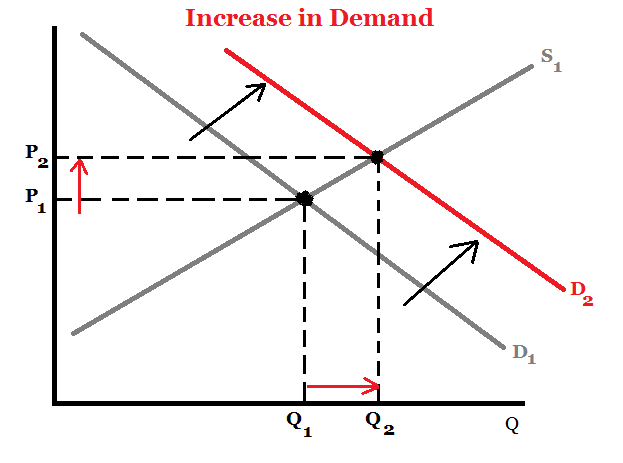
Increase in Demand

If demand increases due to factors such as higher consumer income or changes in preferences, the demand curve shifts to the right. This results in a higher equilibrium price and quantity.

Example:

  • If more consumers want to buy a good (shift in demand to the right), the equilibrium price will rise, and producers will supply more to meet the increased demand.

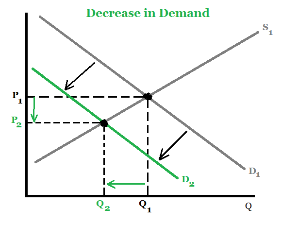
Decrease in Demand

If demand decreases (due to factors such as falling income or changes in preferences), the demand curve shifts to the left. This results in a lower equilibrium price and quantity.

Example:

  • If consumers no longer desire a good, the equilibrium price falls, and producers may reduce the quantity supplied.

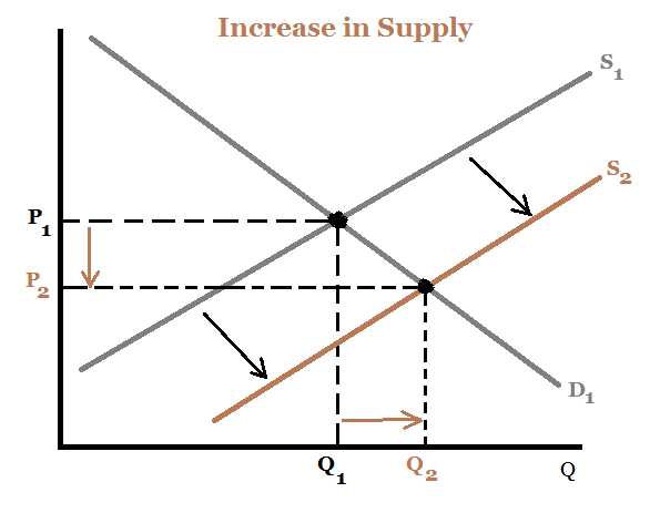
Increase in Supply

If supply increases (due to factors such as technological improvements or lower production costs), the supply curve shifts to the right. This results in a lower equilibrium price and a higher equilibrium quantity.

Example:

  • If a new technology reduces the cost of producing a good, the supply curve shifts rightward, leading to a lower price and higher quantity.

Decrease in Supply

If supply decreases (due to factors such as higher production costs or natural disasters), the supply curve shifts to the left. This results in a higher equilibrium price and a lower equilibrium quantity.

Example:

  • If a natural disaster disrupts the production of a good, the supply decreases, leading to higher prices and lower quantities available.

Role of Price Mechanism in Reaching Equilibrium

The price mechanism plays a crucial role in reaching equilibrium. If there is a surplus (where supply exceeds demand), producers will lower prices to encourage consumers to buy more. Conversely, if there is a shortage (where demand exceeds supply), consumers will compete to buy the good, causing prices to rise. This process continues until the market reaches equilibrium.

  • Surplus: If the price is above equilibrium, supply exceeds demand, and producers reduce the price.
  • Shortage: If the price is below equilibrium, demand exceeds supply, and prices rise as consumers compete for the limited supply.

Shifts in the Supply and Demand Curve

Definitely, if there is any change in supply, demand or both the market equilibrium would change. Let’s recollect the factors that induce changes in demand and supply:

Shift in Demand

The demand for a product changes due to an alteration in any of the following factors:

  • Price of complementary goods
  • Price of substitute goods
  • Income
  • Tastes and preferences
  • An expectation of change in the price in future
  • Population

Shift in Supply

The supply of product changes due to an alteration in any of the following factors:

  • Prices of factors of production
  • Prices of other goods
  • State of technology
  • Taxation policy
  • An expectation of change in price in future
  • Goals of the firm
  • Number of firms

Now let us study individually how market equilibrium changes when only demand changes, only supply changes and when both demand and supply change.

When only Demand Changes

A change in demand can be recorded as either an increase or a decrease. Note that in this case there is a shift in the demand curve.

(i) Increase in Demand

When there is an increase in demand, with no change in supply, the demand curve tends to shift rightwards. As the demand increases, a condition of excess demand occurs at the old equilibrium price. This leads to an increase in competition among the buyers, which in turn pushes up the price.

  • Shifts in Demand and Supply
  • Equilibrium, Excess Demand and Supply

Of course, as price increases, it serves as an incentive for suppliers to increase supply and also leads to a fall in demand. It is important to realize that these processes continue to operate until a new equilibrium is established. Effectively, there is an increase in both the equilibrium price and quantity.

(ii) Decrease in Demand

Under conditions of a decrease in demand, with no change in supply, the demand curve shifts towards left. When demand decreases, a condition of excess supply is built at the old equilibrium level. This leads to an increase in competition among the sellers to sell their produce, which obviously decreases the price.

Now as for price decreases, more consumers start demanding the good or service. Observably, this decrease in price leads to a fall in supply and a rise in demand. This counter mechanism continues until the conditions of excess supply are wiped out at the old equilibrium level and a new equilibrium is established. Effectively, there is a decrease in both the equilibrium price and quantity.

When only Supply Changes

A change in supply can be noted as either an increase or a decrease. Note that in this case there is a shift in the supply curve.

(i) Increase in Supply

When supply increases, accompanied by no change in demand, the supply curve shift towards the right. When supply increases, a condition of excess supply arises at the old equilibrium level. This induces competition among the sellers to sell their supply, which in turn decreases the price.

This decrease in price, in turn, leads to a fall in supply and a rise in demand. These processes operate until a new equilibrium level is attained. Lastly, such conditions are marked by a decrease in price and an increase in quantity.

(ii) Decrease in Supply

When the supply decreases, accompanied by no change in demand, there is a leftward shift of the supply curve. As supply decreases, a condition of excess demand is created at the old equilibrium level. Effectively there is increased competition among the buyers, which obviously leads to a rise in the price.

An increase in price is accompanied by a decrease in demand and an increase in supply. This continues until a new equilibrium level is attained. Further, there is a rise in equilibrium price but a fall in equilibrium quantity.

When both Demand and Supply Change

Generally, the market situation is more complex than the above-mentioned cases. That means, generally, supply and demand do not change in an individual manner. There is a simultaneous change in both entities. This gives birth to four cases:

  • Both demand and supply decrease
  • Both demand and supply increase
  • Demand decreases but supply increases
  • Demand increases but supply decreases

(i) Both Demand and Supply Decrease

The final market conditions can be determined only by a deduction of the magnitude of the decrease in both demand and supply. In fact, both the demand and supply curve shift towards the left. Essentially, there is a need to compare their magnitudes. Such conditions are better analyzed by dividing this case further into three:

The decrease in demand = decrease in supply

When the magnitudes of the decrease in both demand and supply are equal, it leads to a proportionate shift of both demand and supply curve. Consequently, the equilibrium price remains the same but there is a decrease in the equilibrium quantity.

The decrease in demand > decrease in supply

When the decrease in demand is greater than the decrease in supply, the demand curve shifts more towards left relative to the supply curve. Effectively, there is a fall in both equilibrium quantity and price.

The decrease in demand < decrease in supply

In a case in which the decrease in demand is smaller than the decrease in supply, the leftward shift of the demand curve is less than the leftward shift of the supply curve. Notably, there is a rise in equilibrium price accompanied by a fall in equilibrium quantity.

(ii) Both Demand and Supply Increase

In such a condition both demand and supply shift rightwards. So, in order to study changes in market equilibrium, we need to compare the increase in both entities and then conclude accordingly. Such a condition is further studied better with the help of the following three cases:

The increase in demand = increase in supply

If the increase in both demand and supply is exactly equal, there occurs a proportionate shift in the demand and supply curve. Consequently, the equilibrium price remains the same. However, the equilibrium quantity rises.

The increase in demand > increase in supply

In such a case, the right shift of the demand curve is more relative to that of the supply curve. Effectively, both equilibrium price and quantity tend to increase.

The increase in demand < increase in supply

When the increase is demand is less than the increase in supply, the right shift of the demand curve is less than the right shift of supply curve. In this case, the equilibrium price falls whereas the equilibrium quantity rises.

(iii) Demand Decreases but Supply Increases

This condition translates to the fact that the demand curve shifts leftwards whereas the supply curve shifts rightwards. As they move in opposite directions, the final market conditions are deduced by pointing out the magnitude of their shifts. Here, three cases further arise which are as follows:

The decrease in demand = increase in supply

In this case, although the two curves move in opposite directions, the magnitudes of their shifts is effectively the same. As a result, the equilibrium quantity remains the same but the equilibrium price falls.

The decrease in demand > increase in supply

When the decrease in demand is greater than the increase in supply, the relative shift of demand curve is proportionately more than the supply curve. Effectively, both the equilibrium quantity and price fall.

The decrease in demand < increase in supply

Here, the leftward shift of the demand curve is less than the rightward shift of the supply curve. It is important to realize, that the equilibrium quantity rises whereas the equilibrium price falls.

(iv) Demand Increases but Supply Decreases

Similar to the aforementioned condition, here also the demand and supply curve moves in the opposite directions. However, the demand curve shift towards the right(indicating an increase in demand) and the supply curve shift towards left(indicating a decrease in supply). Further, this is studied with the help of the following three cases:

Increase in demand = decrease in supply

When the increase in demand is equal to the decrease in supply, the shifts in both supply and demand curves are proportionately equal. Effectively, the equilibrium quantity remains the same however the equilibrium price rises.

Increase in demand > decrease in supply

In this case, the right shift of the demand curve is proportionately more than the leftward shift of the supply curve. Hence, both equilibrium quantity and price rise.

Increase in demand < decrease in supply

If the increase in demand is less than the decrease in supply, the shift of the demand curve tends to be less than that of the supply curve. Effectively, equilibrium quantity falls whereas the equilibrium price rises.

Demand Estimation and Forecasting

Demand Estimation is the process of predicting the future demand for a product or service based on historical data, market trends, and influencing factors. It involves analyzing variables such as price, income levels, population, consumer preferences, and substitute goods to determine the quantity consumers are likely to purchase. Demand estimation is crucial for businesses to plan production, set prices, allocate resources efficiently, and develop strategies for market penetration. Methods include statistical techniques, surveys, and econometric models. Accurate demand estimation helps minimize risks, reduce costs, and align supply with anticipated consumer needs, ensuring better decision-making and market competitiveness.

Demand Forecasting refers to the process of predicting future consumer demand for a product or service over a specific period. It is based on the analysis of historical sales data, market trends, and external factors like economic conditions, seasonal variations, and industry developments. Businesses use demand forecasting to make informed decisions about production planning, inventory management, staffing, and financial budgeting. Techniques include qualitative methods like expert opinion and quantitative approaches such as time-series analysis and regression models. Accurate forecasting helps companies meet customer demand efficiently, avoid overproduction or stockouts, and improve overall operational and financial performance.

1. Survey Methods

Survey methods are qualitative approaches that gather firsthand information from consumers, experts, or market participants. These methods are particularly useful for new products or when historical data is unavailable.

Techniques in Survey Methods

  1. Consumer Survey

    • Directly asks consumers about their future purchasing intentions.
    • Methods include interviews, questionnaires, or focus groups.
    • Effective for products with short purchase cycles or in small markets.
  2. Sales Force Opinion

    • Relies on the insights of sales representatives who interact with customers.
    • Aggregates predictions from sales teams to estimate demand.
    • Useful when sales teams have a deep understanding of customer behavior.
  3. Expert Opinion (Delphi Method)

    • Gathers insights from industry experts or specialists.
    • Repeated rounds of discussion refine estimates, leading to consensus.
    • Best for forecasting in industries with rapid technological changes.
  4. Market Experimentation

    • Tests demand by introducing the product in a limited market or under controlled conditions.
    • Provides empirical data for forecasting in wider markets.

Advantages

  • Provides real-time and targeted information.
  • Particularly helpful for new products or industries.
  • Easy to adapt to specific markets or customer segments.

Limitations

  • Expensive and time-consuming, especially for large-scale surveys.
  • Responses may be biased or inaccurate.
  • Results are often subjective and less reliable for long-term forecasts.

2. Statistical Methods

Statistical methods use quantitative techniques to analyze historical data and predict future demand. These methods are preferred for established products with available historical data.

Techniques in Statistical Methods

  1. Time-Series Analysis

    • Studies historical data to identify patterns or trends.
    • Techniques include moving averages, exponential smoothing, and seasonal decomposition.
    • Suitable for stable markets with predictable demand cycles.
  2. Regression Analysis

    • Examines relationships between demand (dependent variable) and influencing factors (independent variables like price, income, or advertising).
    • Helps identify key determinants of demand and predict changes based on these factors.
  3. Trend Projection

    • Extends historical trends into the future using graphical or mathematical methods.
    • Simple and effective for products with consistent growth or decline patterns.
  4. Econometric Models

    • Builds complex models using economic theories to predict demand.
    • Incorporates multiple variables and interdependencies.
    • Useful for detailed analysis and policy evaluation.
  5. Seasonal Index

    • Adjusts forecasts to account for seasonal variations in demand.
    • Common in industries like retail, tourism, and agriculture.

Advantages

  • Based on objective and reliable data.
  • Effective for long-term and large-scale forecasting.
  • Provides quantifiable and reproducible results.

Limitations

  • Requires accurate and extensive historical data.
  • Assumes past patterns will continue in the future, which may not hold true.
  • Complex methods may require expertise and advanced tools.

Indifference Curve Analysis

Indifference curve analysis is basically an attempt to improve cardinal utility analysis (principle of marginal utility). The cardinal utility approach, though very useful in studying elementary consumer behavior, is criticized for its unrealistic assumptions vehemently. In particular, economists such as Edgeworth, Hicks, Allen and Slutsky opposed utility as a measurable entity. According to them, utility is a subjective phenomenon and can never be measured on an absolute scale. The disbelief on the measurement of utility forced them to explore an alternative approach to study consumer behavior. The exploration led them to come up with the ordinal utility approach or indifference curve analysis. Because of this reason, aforementioned economists are known as ordinalists. As per indifference curve analysis, utility is not a measurable entity. However, consumers can rank their preferences.

Indifference Curve Analysis Vs. Marginal Utility Approach

Let us look at a simple example. Suppose there are two commodities, namely apple and orange. The consumer has $10. If he spends entire money on buying apple, it means that apple gives him more satisfaction than orange. Thus, in indifference curve analysis, we conclude that the consumer prefers apple to orange. In other words, he ranks apple first and orange second. However, in cardinal or marginal utility approach, the utility derived from apple is measured (for example, 10 utils). Similarly, the utility derived from orange is measured (for example, 5 utils). Now the consumer compares both and prefers the commodity that gives higher amount of utility. Indifference curve analysis strictly says that utility is not a measurable entity. What we do here is that we observe what the consumer prefers and conclude that the preferred commodity (apple in our example) gives him more satisfaction. We never try to answer ‘how much satisfaction (utility)’ in indifference curve analysis.

Assumptions

Theories of economics cannot survive without assumptions and indifference curve analysis is no different. The following are the assumptions of indifference curve analysis:

  • Rationality

The theory of indifference curve studies consumer behavior. In order to derive a plausible conclusion, the consumer under consideration must be a rational human being. For example, there are two commodities called ‘A’ and ‘B’. Now the consumer must be able to say which commodity he prefers. The answer must be a definite. For instance – ‘I prefer A to B’ or ‘I prefer B to A’ or ‘I prefer both equally’. Technically, this assumption is known as completeness or trichotomy assumption.

  • Consistency

Another important assumption is consistency. It means that the consumer must be consistent in his preferences. For example, let us consider three different commodities called ‘A’, ‘B’ and ‘C’. If the consumer prefers A to B and B to C, obviously, he must prefer A to C. In this case, he must not be in a position to prefer C to A since this decision becomes self-contradictory.

Symbolically,

If A > B, and B > c, then A > C.

  • More Goods to Less

The indifference curve analysis assumes that consumer always prefers more goods to less. Suppose there are two bundles of commodities – ‘A’ and ‘B’. If bundle A has more goods than bundle B, then the consumer prefers bundle A to B.

  • Substitutes and Complements

In indifference curve analysis, there exist substitutes and complements for the goods preferred by the consumer. However, in marginal utility approach, we assume that goods under consideration do not have substitutes and complements.

  • Income and Market Prices

Finally, the consumer’s income and prices of commodities are fixed. In other words, with given income and market prices, the consumer tries to maximize utility.

  • Indifference Schedule

An indifference schedule is a list of various combinations of commodities that give equal satisfaction or utility to consumers. For simplicity, we have considered only two commodities, ‘X’ and ‘Y’, in our Table 1. Table 1 shows various combinations of X and Y; however, all these combinations give equal satisfaction (k) to the consumer.

Table 1: Indifference Schedule

Combinations X (Oranges) Y (Apples) Satisfaction
A 2 15 k
B 5 9 k
C 7 6 k
D 17 2 k

You can construct an indifference curve from an indifference schedule in the same way you construct a demand curve from a demand schedule.

On the graph, the locus of all combinations of commodities (X and Y in our example) forms an indifference curve (figure 1). Movement along the indifference curve gives various combinations of commodities (X and Y); however, yields same level of satisfaction. An indifference curve is also known as iso utility curve (“iso” means same). A set of indifference curves is known as an indifference map.

Marginal Rate of Substitution

Marginal rate of substitution is an eminent concept in the indifference curve analysis. Marginal rate of substitution tells you the amount of one commodity the consumer is willing to give up for an additional unit of another commodity. In our example (table 1), we have considered commodity X and Y. Hence, the marginal rate of substitution of X for Y (MRSxy) is the maximum amount of Y the consumer is willing to give up for an additional unit of X. However, the consumer remains on the same indifference curve.

In other words, the marginal rate of substitution explains the tradeoff between two goods.

Diminishing marginal rate of substitution

From table 1 and figure 1, we can easily explain the concept of diminishing marginal rate of substitution. In our example, we substitute commodity X for commodity Y. Hence, the change in Y is negative (i.e., -ΔY) since Y decreases.

Thus, the equation is

MRSxy = -ΔY/ΔX and

MRSyx = -ΔX/ΔY

However, convention is to ignore the minus sign; hence,

MRSxy = ΔY/ΔX

In figure 1, X denotes oranges and Y denotes apples. Points A, B, C and D indicate various combinations of oranges and apples.

In this example, we have the following marginal rate of substitution:

MRSx for y between A and B: AA­­1/A1B = 6/3 = 2.0

MRSx for y between B and C: BB­­1/B1C = 3/2 = 1.5

MRSx for y between C and D: CC­­1/C1D = 4/10 = 0.4

Thus, MRSx for y diminishes for every additional units of X. This is the principle of diminishing marginal rate of substitution.

Law of Demand

Demand theory is a principle relating to the relationship between consumer demand for goods and services and their prices. Demand theory forms the basis for the demand curve, which relates consumer desire to the amount of goods available. As more of a good or service is available, demand drops and so does the equilibrium price.

Demand is the quantity of a good or service that consumers are willing and able to buy at a given price in a given time period. People demand goods and services in an economy to satisfy their wants, such as food, healthcare, clothing, entertainment, shelter, etc. The demand for a product at a certain price reflects the satisfaction that an individual expects from consuming the product. This level of satisfaction is referred to as utility and it differs from consumer to consumer. The demand for a good or service depends on two factors:

  • Its utility to satisfy a want or need.
  • The consumer’s ability to pay for the good or service. In effect, real demand is when the readiness to satisfy a want is backed up by the individual’s ability and willingness to pay.

Built into demand are factors such as consumer preferences, tastes, choices, etc. Evaluating demand in an economy is, therefore, one of the most important decision-making variables that a business must analyze if it is to survive and grow in a competitive market. The market system is governed by the laws of supply and demand, which determine the prices of goods and services. When supply equals demand, prices are said to be in a state of equilibrium. When demand is higher than supply, prices increase to reflect scarcity. Conversely, when demand is lower than supply, prices fall due to the surplus.

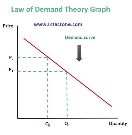
The law of demand introduces an inverse relationship between price and demand for a good or service. It simply states that as the price of a commodity increases, demand decreases, provided other factors remain constant. Also, as the price decreases, demand increases. This relationship can be illustrated graphically using a tool known as the demand curve.

The demand curve has a negative slope as it charts downward from left to right to reflect the inverse relationship between the price of an item and the quantity demanded over a period of time. An expansion or contraction of demand occurs as a result of the income effect or substitution effect. When the price of a commodity falls, an individual can get the same level of satisfaction for less expenditure, provided it’s a normal good. In this case, the consumer can purchase more of the goods on a given budget. This is the income effect. The substitution effect is observed when consumers switch from more costly goods to substitutes that have fallen in price. As more people buy the good with the lower price, demand increases.

Sometimes, consumers buy more or less of a good or service due to factors other than price. This is referred to as a change in demand. A change in demand refers to a shift in the demand curve to the right or left following a change in consumers’ preferences, taste, income, etc. For example, a consumer who receives an income raise at work will have more disposable income to spend on goods in the markets, regardless of whether prices fall, leading to a shift to the right of the demand curve.

The law of demand is violated when dealing with Giffen or inferior goods. Giffen goods are inferior goods that people consume more of as prices rise, and vice versa. Since a Giffen good does not have easily available substitutes, the income effect dominates the substitution effect.

Demand theory is one of the core theories of microeconomics. It aims to answer basic questions about how badly people want things, and how demand is impacted by income levels and satisfaction (utility). Based on the perceived utility of goods and services by consumers, companies adjust the supply available and the prices charged.

Law of Demand

The law of demand is one of the most fundamental concepts in economics. It works with the law of supply to explain how market economies allocate resources and determine the prices of goods and services that we observe in everyday transactions. The law of demand states that quantity purchased varies inversely with price. In other words, the higher the price, the lower the quantity demanded. This occurs because of diminishing marginal utility. That is, consumers use the first units of an economic good they purchase to serve their most urgent needs first, and use each additional unit of the good to serve successively lower valued ends.

  • The law of demand is a fundamental principle of economics which states that at a higher price consumers will demand a lower quantity of a good.
  • Demand is derived from the law of diminishing marginal utility, the fact that consumers use economic goods to satisfy their most urgent needs first.
  • A market demand curve expresses the sum of quantity demanded at each price across all consumers in the market.
  • Changes in price can be reflected in movement along a demand curve, but do not by themselves increase or decrease demand.
  • The shape and magnitude of demand shifts in response to changes in consumer preferences, incomes, or related economic goods, NOT to changes in price.

Understanding the Law of Demand

Economics involves the study of how people use limited means to satisfy unlimited wants. The law of demand focuses on those unlimited wants. Naturally, people prioritize more urgent wants and needs over less urgent ones in their economic behavior, and this carries over into how people choose among the limited means available to them. For any economic good, the first unit of that good that a consumer gets their hands on will tend to be put to use to satisfy the most urgent need the consumer has that that good can satisfy.

For example, consider a castaway on a desert island who obtains a six pack of bottled, fresh water washed up on shore. The first bottle will be used to satisfy the castaway’s most urgently felt need, most likely drinking water to avoid dying of thirst. The second bottle might be used for bathing to stave off disease, an urgent but less immediate need. The third bottle could be used for a less urgent need such as boiling some fish to have a hot meal, and on down to the last bottle, which the castaway uses for a relatively low priority like watering a small potted plant to keep him company on the island.

In our example, because each additional bottle of water is used for a successively less highly valued want or need by our castaway, we can say that the castaway values each additional bottle less than the one before. Similarly, when consumers purchase goods on the market each additional unit of any given good or service that they buy will be put to a less valued use than the one before, so we can say that they value each additional unit less and less. Because they value each additional unit of the good less, they are willing to pay less for it. So the more units of a good consumers buy, the less they are willing to pay in terms of the price.

By adding up all the units of a good that consumers are willing to buy at any given price we can describe a market demand curve, which is always downward-sloping, like the one shown in the chart below. Each point on the curve (A, B, C) reflects the quantity demanded (Q) at a given price (P). At point A, for example, the quantity demanded is low (Q1) and the price is high (P1). At higher prices, consumers demand less of the good, and at lower prices, they demand more.

Factors Affecting Demand

The shape and position of the demand curve can be impacted by several factors. Rising incomes tend to increase demand for normal economic goods, as people are willing to spend more. The availability of close substitute products that compete with a given economic good will tend to reduce demand for that good, since they can satisfy the same kinds of consumer wants and needs. Conversely, the availability of closely complementary goods will tend to increase demand for an economic good, because the use of two goods together can be even more valuable to consumers than using them separately, like peanut butter and jelly. Other factors such as future expectations, changes in background environmental conditions, or change in the actual or perceived quality of a good can change the demand curve, because they alter the pattern of consumer preferences for how the good can be used and how urgently it is needed.

Demand theory objectives

  • Forecasting sales
  • Ma­nipulating demand
  • Appraising salesmen’s performance for setting their sales quotas
  • Watching the trend of the company’s competi­tive position.

Of these the first two are most im­portant and the last two are ancillary to the main economic problem of planning for profit.

1. Forecasting Demand

Forecasting refers to predicting the future level of sales on the basis of current and past trends. This is perhaps the most important use of demand stud­ies. True, sales forecast is the foundation for plan­ning all phases of the company’s operations. There­fore, purchasing and capital budget (expenditure) programmes are all based on the sales forecast.

2. Manipulating Demand

Sales forecasting is most passive. Very few com­panies take full advantage of it as a technique for formulating business plans and policies. However, “management must recognize the degree to which sales are a result only of the external economic environment but also of the action of the company itself.

Sales volumes do differ, “depending upon how much money is spent on advertising, what price policy is adopted, what product improve­ments are made, how accurately salesmen and sales efforts are matched with potential sales in the various territories, and so forth”.

Often advertising is intended to change consumer tastes in a manner favourable to the advertiser’s product. The efforts of so-called ‘hidden persuaders’ are directed to ma­nipulate people’s ‘true’ wants. Thus sales forecasts should be used for estimating the consequences of other plans for adjusting prices, promotion and/or products.

Importance of Demand Analysis

  • Business Forecasting

Demand analysis is vital for forecasting future sales. It helps businesses estimate the quantity of a product that consumers will likely purchase over a specific period. Accurate forecasts enable companies to plan production schedules, manage inventory, allocate resources efficiently, and avoid underproduction or overproduction. This proactive planning improves operational efficiency and reduces costs. Demand forecasting also helps firms adapt to seasonal changes, market trends, and economic fluctuations, ensuring they remain responsive to consumer needs and market conditions.

  • Pricing Policy Formulation

Understanding demand is essential for determining the most effective pricing strategy. Through demand analysis, firms can identify how sensitive consumers are to price changes (price elasticity of demand). If demand is inelastic, companies may raise prices without a significant drop in sales. If it is elastic, firms must remain competitive with pricing. Analyzing demand patterns helps in setting optimal prices that balance profitability with consumer satisfaction, ensuring maximum revenue without alienating potential buyers.

  • Efficient Resource Allocation

Demand analysis aids in the optimal allocation of limited resources. By knowing which products or services are in high demand, businesses can prioritize investments, labor, and raw materials accordingly. This ensures resources are not wasted on low-demand items. For example, if demand analysis shows growing interest in electric vehicles, manufacturers may divert resources from traditional models to electric production, leading to better financial returns and strategic growth.

  • Marketing and Sales Strategy Development

An effective marketing plan depends on a deep understanding of consumer demand. Demand analysis reveals who the buyers are, what they need, and how much they are willing to spend. Businesses can tailor promotions, distribution channels, and product features to match demand patterns. Targeted campaigns and personalized customer engagement strategies become more effective when rooted in accurate demand insights, leading to higher conversion rates and customer loyalty.

  • Product Planning and Development

Demand analysis supports product innovation and development decisions. It helps firms identify unmet needs and emerging trends in the market. By studying demand data, companies can decide whether to introduce new products, discontinue existing ones, or modify features to meet changing customer preferences. This reduces the risk of product failure and increases the chances of launching offerings that are relevant, timely, and well-received by consumers.

  • Investment Decision-Making

Before investing in new plants, equipment, or market expansion, companies need to assess whether future demand justifies such expenditure. Demand analysis provides the necessary insights to evaluate potential returns on investment. For example, if demand is expected to grow significantly in a region, it may warrant establishing a new facility there. This minimizes financial risk and aligns investment decisions with long-term market opportunities and consumer behavior.

  • Helps Government and Policy Makers

Governments and policy makers use demand analysis to make informed decisions about infrastructure, subsidies, taxes, and social welfare programs. By understanding what goods and services are in high demand, governments can align public spending with citizen needs. Demand insights also aid in controlling inflation, managing subsidies, and framing import-export policies. For instance, demand data for housing or healthcare helps governments prioritize urban development and public service improvements.

  • Risk Management and Contingency Planning

Demand analysis helps businesses identify potential risks associated with market fluctuations. By studying demand trends, companies can anticipate downturns, supply disruptions, or changing customer preferences. This allows them to develop contingency plans, diversify offerings, or explore new markets in advance. For example, if a drop in demand for fossil fuels is predicted, energy firms can pivot toward renewables. Thus, demand analysis minimizes uncertainty and enhances long-term sustainability.

Law of Diminishing Marginal utility

Law of Diminishing Marginal Utility states that as a person consumes additional units of a good or service, the satisfaction (utility) derived from each successive unit decreases, assuming all other factors remain constant. Initially, the first few units provide significant satisfaction, but as consumption increases, the utility of each extra unit diminishes. For example, the first slice of pizza may bring great joy, but by the fifth or sixth slice, the additional satisfaction reduces. This principle underlies consumer behavior and helps explain demand curves, as consumers are less willing to pay the same price for additional units of a product.

Assumptions:

Following are the assumptions of the law of diminishing marginal utility.

  1. The utility is measurable and a person can express the utility derived from a commodity in qualitative terms such as 2 units, 4 units and 7 units etc.
  2. A rational consumer aims at the maximization of his utility.
  3. It is necessary that a standard unit of measurement is constant
  4. A commodity is being taken continuously. Any gap between the consumption of a commodity should be suitable.
  5. There should be proper units of a good consumed by the consumer.
  6. It is assumed that various units of commodity homogeneous in characteristics.
  7. The taste of the consumer remains same during the consumption o the successive units of commodity.
  8. Income of the consumer remains constant during the operation of the law of diminishing marginal utility.
  9. It is assumed that the commodity is divisible.
  • There should be not change in fashion. For example, if there is a fashion of lifted shirts, then the consumer may have no utility in open shirts.
  • It is assumed that the prices of the substitutes do not change. For example, the demand for CNG increases due to rise in the prices of petroleum and these price changes effect the utility of CNG.

Explanation with Schedule and Diagram:

We assume that a man is very thirsty. He takes the glasses of water successively. The marginal utility of the successive glasses of water decreases, ultimately, he reaches the point of satiety. After this point the marginal utility becomes negative, if he is forced further to take a glass of water. The behavior of the consumer is indicated in the following schedule:

Units of commodity Marginal utility Total utility
1st glass 10 10
2nd glass 8 18
3rd glass 6 24
4th glass 4 28
5th glass 2 30
6th glass 0 30
7th glass -2 28

On taking the 1st glass of water, the consumer gets 10 units of utility, because he is very thirsty. When he takes 2nd glass of water, his marginal utility goes down to 8 units because his thirst has been partly satisfied. This process continues until the marginal utility drops down to zero which is the saturation point. By taking the seventh glass of water, the marginal utility becomes negative because the thirst of the consumer has already been fully satisfied.

The law of diminishing marginal utility can be explained by the following diagram drawn with the help of above schedule:

9.1.png

In the above figure, the marginal utility of different glasses of water is measured on the y-axis and the units (glasses of water) on X-axis. With the help of the schedule, the points A, B, C, D, E, F and G are derived by the different combinations of units of the commodity (glasses of water) and the marginal utility gained by different units of commodity. By joining these points, we get the marginal utility curve. The marginal utility curve has the downward negative slope. It intersects the X-axis at the point of 6th unit of the commodity. At this point “F” the marginal utility becomes zero. When the MU curve goes beyond this point, the MU becomes negative. So there is an inverse functional relationship between the units of a commodity and the marginal utility of that commodity.

Exceptions or Limitations:

The limitations or exceptions of the law of diminishing marginal utility are as follows:

  1. The law does not hold well in the rare collections. For example, collection of ancient coins, stamps etc.
  2. The law is not fully applicable to money. The marginal utility of money declines with richness but never falls to zero.
  3. It does not apply to the knowledge, art and innovations.
  4. The law is not applicable for precious goods.
  5. Historical things are also included in exceptions to the law.
  6. Law does not operate if consumer behaves in irrational manner. For example, drunkard is said to enjoy each successive peg more than the previous one.
  7. Man is fond of beauty and decoration. He gets more satisfaction by getting the above merits of the commodities.
  8. If a dress comes in fashion, its utility goes up. On the other hand its utility goes down if it goes out of fashion.
  9. The utility increases due to demonstration. It is a natural element.

Importance of the Law of Diminishing Marginal Utility:

  1. By purchasing more of a commodity the marginal utility decreases. Due to this behaviour, the consumer cuts his expenditures to that commodity.
  2. In the field of public finance, this law has a practical application, imposing a heavier burden on the rich people.
  3. This law is the base of some other economic laws such as law of demand, elasticity of demand, consumer surplus and the law of substitution etc.
  4. The value of commodity falls by increasing the supply of a commodity. It forms a basis of the theory of value. In this way prices are determined

Equi Marginal Utility

Equi-Marginal Principle (also known as the principle of equal marginal utility or the law of equi-marginal utility) is a fundamental concept in economics that helps individuals and businesses maximize satisfaction or profit. According to this principle, resources should be allocated in such a way that the marginal utility or marginal returns from each resource are equal across all possible uses.

In other words, whether a consumer is trying to maximize their utility or a firm is trying to maximize profit, they will distribute their limited resources (money, labor, time, etc.) among various alternatives so that the additional (marginal) benefit derived from the last unit of resource used in each alternative is equal.

Key Elements of the Equi-Marginal Principle:

  1. Marginal Utility:

Marginal utility refers to the additional satisfaction or benefit that a person receives from consuming an additional unit of a good or service. As more of a good is consumed, the marginal utility usually decreases, a concept known as diminishing marginal utility.

  1. Marginal Productivity/Returns:

In business, marginal productivity or marginal returns refer to the additional output that can be obtained by using an additional unit of input. Like marginal utility, marginal returns also generally diminish as more units of input are added.

  1. Optimization:

The equi-marginal principle is about optimization. Consumers aim to allocate their resources (income) in such a way that the marginal utility per unit of money spent is equal for all goods. Similarly, firms allocate inputs like labor and capital to maximize profit, ensuring that the marginal returns from each input are equal across all uses.

Formula for the Equi-Marginal Principle

For consumers: The formula for maximizing utility using the equi-marginal principle is as follows:

8.2

Example: Allocation of Consumer Budget

Let’s assume a consumer has a budget of $100 to spend on two goods, A and B. The consumer’s goal is to allocate their budget in such a way that the total utility derived from consuming both goods is maximized.

Table of Marginal Utility and Price:

Units Consumed Marginal Utility of A (MUA​) Price of A (PA​) MUA​/PA​ Marginal Utility of B (MUB​) Price of B (PB​) MUB​/PB​
1 20 $10 2 24 $8 3
2 18 $10 1.8 20 $8 2.5
3 16 $10 1.6 16 $8 2
4 14 $10 1.4 12 $8 1.5
5 12 $10 1.2 8 $8 1

From the table, we can see the marginal utility per dollar spent on each good for various levels of consumption.

Allocation Process:

  1. Initially, the consumer will compare the MU/P ratios for both goods.
  2. The consumer will spend their first dollar on Good B because it provides a higher marginal utility per dollar (3) than Good A (2).
  3. After consuming the first unit of Good B, the consumer will compare the MU/P ratios again. Since MUB/PB=2.5 is still higher than MUA/PA=2, the consumer will purchase another unit of Good B.
  4. This process will continue until the MU/P ratios for both goods are equal or the consumer’s budget is exhausted.

In this case, the consumer might end up purchasing 2 units of Good A and 3 units of Good B, at which point the marginal utility per dollar for both goods becomes approximately equal, maximizing their total utility.

Example: Firm’s Input Allocation

Let’s assume a firm has two inputs: labor (L) and capital (K). The firm wants to allocate these inputs to maximize profit, with the marginal product and cost data as follows:

Input Marginal Product of Labor (MPL​) Cost of Labor (CL) MPL​/CL​ Marginal Product of Capital (MPK​) Cost of Capital (CK​) MPK​/CK​
1 50 $10 5 80 $20 4
2 40 $10 4 70 $20 3.5
3 30 $10 3 60 $20 3
4 20 $10 2 50 $20 2.5
5 10 $10 1 40 $20 2

The firm’s goal is to allocate labor and capital in such a way that the marginal product per unit of cost is equal for both inputs.

Allocation Process:

  1. Initially, the firm compares the MP/C ratios for labor and capital.
  2. The firm will allocate its first dollar towards labor, where MPL/CL=5 is greater than MPK/CK=4.
  3. After allocating more resources, the firm will continue comparing the ratios.
  4. The firm will keep allocating resources until the marginal product per unit cost for both labor and capital is equal.

In this case, the optimal allocation would involve using 2 units of labor and 1 unit of capital, where the marginal products per unit cost are equal (4), maximizing the firm’s profit.

Importance of the Equi-Marginal Principle:

  • Efficient Allocation:

The equi-marginal principle ensures the efficient allocation of resources, whether for consumers aiming to maximize utility or firms aiming to maximize profit. By allocating resources where they provide the highest marginal benefit, both individuals and businesses can make the best possible use of their limited resources.

  • Economic Decision-Making:

This principle is a key component of rational decision-making in economics. It helps in determining the optimal quantity of goods to consume, the best mix of inputs to use in production, or even the best way to allocate time among different activities.

  • Flexibility:

The equi-marginal principle can be applied across various fields of economics, from consumer theory and production theory to cost minimization and utility maximization.

Explanation of the Law:

In order to get maximum satisfaction out of the funds we have, we carefully weigh the satisfaction obtained from each rupee ‘had we spend If we find that a rupee spent in one direction has greater utility than in another, we shall go on spending money on the former commodity, till the satisfaction derived from the last rupee spent in the two cases is equal.

It other words, we substitute some units of the commodity of greater utility tor some units of the commodity of less utility. The result of this substitution will be that the marginal utility of the former will fall and that of the latter will rise, till the two marginal utilities are equalized. That is why the law is also called the Law of Substitution or the Law of equimarginal Utility.

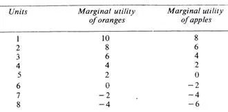
Suppose apples and oranges are the two commodities to be purchased. Suppose further that we have got seven rupees to spend. Let us spend three rupees on oranges and four rupees on apples. What is the result? The utility of the 3rd unit of oranges is 6 and that of the 4th unit of apples is 2. As the marginal utility of oranges is higher, we should buy more of oranges and less of apples. Let us substitute one orange for one apple so that we buy four oranges and three apples.

Now the marginal utility of both oranges and apples is the same, i.e., 4. This arrangement yields maximum satisfaction. The total utility of 4 oranges would be 10 + 8 + 6 + 4 = 28 and of three apples 8 + 6 + 4= 18 which gives us a total utility of 46. The satisfaction given by 4 oranges and 3 apples at one rupee each is greater than could be obtained by any other combination of apples and oranges. In no other case does this utility amount to 46. We may take some other combinations and see.

We thus come to the conclusion that we obtain maximum satisfaction when we equalize marginal utilities by substituting some units of the more useful for the less useful commodity. We can illustrate this principle with the help of a diagram.

Diagrammatic Representation:

In the two figures given below, OX and OY are the two axes. On X-axis OX are represented the units of money and on the Y-axis marginal utilities. Suppose a person has 7 rupees to spend on apples and oranges whose diminishing marginal utilities are shown by the two curves AP and OR respectively.

The consumer will gain maximum satisfaction if he spends OM money (3 rupees) on apples and OM’ money (4 rupees) on oranges because in this situation the marginal utilities of the two are equal (PM = P’M’). Any other combination will give less total satisfaction.

Let the purchase spend MN money (one rupee) more on apples and the same amount of money, N’M'( = MN) less on oranges. The diagram shows a loss of utility represented by the shaded area LN’M’P’ and a gain of PMNE utility. As MN = N’M’ and PM=P’M’, it is proved that the area LN’M’P’ (loss of utility from reduced consumption of oranges) is bigger than PMNE (gain of utility from increased consumption of apples). Hence the total utility of this new combination is less.

We then, conclude that no other combination of apples and oranges gives as great a satisfaction to the consumer as when PM = P’M’, i.e., where the marginal utilities of apples and oranges purchased are equal, with given amour, of money at our disposal.

Limitations of the Law of Equi-marginal Utility

Like other economic laws, the law of equimarginal utility too has certain limitations or exceptions. The following are the main exception.

(i) Ignorance

If the consumer is ignorant or blindly follows custom or fashion, he will make a wrong use of money. On account of his ignorance he may not know where the utility is greater and where less. Thus, ignorance may prevent him from making a rational use of money. Hence, his satisfaction may not be the maximum, because the marginal utilities from his expenditure can­not be equalised due to ignorance.

(ii) Inefficient Organisation

In the same manner, an incompetent organ­iser of business will fail to achieve the best results from the units of land, labour and capital that he employs. This is so because he may not be able to divert expenditure to more profitable channels from the less profitable ones.

(iii) Unlimited Resources

The law has obviously no place where this resources are unlimited, as for example, is the case with the free gifts of nature. In such cases, there is no need of diverting expenditure from one direction to another.

(iv) Hold of Custom and Fashion

A consumer may be in the strong clutches of custom, or is inclined to be a slave of fashion. In that case, he will not be able to derive maximum satisfaction out of his expenditure, because he cannot give up the consumption of such commodities. This is specially true of the conventional necessaries like dress or when a man is addicted to some into­xicant.

(v) Frequent Changes in Prices

Frequent changes in prices of different goods render the observance of the law very difficult. The consumer may not be able to make the necessary adjustments in his expenditure in a constantly changing price situation.

Key differences between Micro economics and Macro economics

Micro Economics

Microeconomics studies the behavior and decision-making processes of individual consumers and firms. It focuses on how they allocate scarce resources to maximize utility and profit, respectively. Key concepts include supply and demand, market equilibrium, elasticity, and marginal analysis. Microeconomics examines how factors such as price changes, consumer preferences, and production costs affect the choices of buyers and sellers. It also explores market structures—like perfect competition, monopoly, and oligopoly—and their impact on pricing and output. By analyzing these components, microeconomics helps understand how markets function and how individual decisions influence economic outcomes.

Features of Micro Economics:

  1. Individual Decision-Making

Microeconomics centers on how individuals and firms make choices regarding the allocation of their limited resources. It examines consumer behavior, including how preferences and budget constraints influence purchasing decisions, and firm behavior, focusing on production choices and cost management. This feature helps understand the rationale behind personal and business decisions.

  1. Supply and Demand Analysis

A fundamental feature of microeconomics is the study of supply and demand. It explores how these forces interact to determine prices and quantities in individual markets. Demand refers to consumer willingness and ability to purchase goods, while supply pertains to the quantity producers are willing to offer. The equilibrium point, where supply equals demand, is crucial for understanding market dynamics.

  1. Price Mechanism

Microeconomics investigates how prices are determined in various market structures. It looks at how changes in supply and demand affect prices and how prices signal to producers and consumers about resource allocation. The price mechanism helps in understanding how markets clear and how resources are efficiently allocated based on market signals.

  1. Elasticity

Elasticity measures how sensitive the quantity demanded or supplied of a good is to changes in price or other factors. Microeconomics studies price elasticity of demand, income elasticity, and cross-price elasticity, which helps determine how changes in prices, consumer income, or the prices of related goods affect market behavior.

  1. Market Structures

Microeconomics analyzes different market structures, including perfect competition, monopoly, monopolistic competition, and oligopoly. Each structure has unique characteristics regarding the number of firms, product differentiation, and pricing power. Understanding these structures helps explain variations in market outcomes and competitive strategies.

  1. Marginal Analysis

Marginal analysis is a key feature where decisions are made based on marginal changes. It involves examining the additional benefit (marginal benefit) and additional cost (marginal cost) of a decision to determine the optimal level of production or consumption. This analysis helps in maximizing profit or utility.

  1. Consumer Theory

Consumer theory explores how individuals make consumption choices to maximize their utility given their budget constraints. It involves analyzing indifference curves and budget constraints to understand how consumers allocate their income among various goods and services to achieve the highest satisfaction.

  1. Production and Costs

Microeconomics examines how firms produce goods and services and the associated costs. It includes the study of production functions, which describe the relationship between input factors and output, and cost structures, such as fixed and variable costs. This feature helps in understanding how firms optimize production and manage costs to maximize profit.

Macro Economics

Macroeconomics examines the economy as a whole, focusing on aggregate phenomena and large-scale economic factors. Key concepts include Gross Domestic Product (GDP), inflation, unemployment, and national income. It explores how these aggregate variables interact and influence each other, and assesses the overall health and performance of an economy. Macroeconomics also studies fiscal and monetary policies—such as government spending, taxation, and central bank interest rates—and their impact on economic growth, stability, and employment. By analyzing these broad economic indicators, macroeconomics aims to understand and manage economic fluctuations and promote overall economic well-being.

Features of Macro Economics:

  1. Aggregate Indicators

Macroeconomics examines aggregate indicators such as Gross Domestic Product (GDP), inflation rate, unemployment rate, and national income. These indicators provide a comprehensive view of the overall economic performance and health, helping policymakers and economists understand economic trends and conditions.

  1. Economic Growth

A central focus of macroeconomics is understanding and promoting economic growth. It analyzes factors that contribute to increases in a country’s productive capacity over time, such as technological advancements, capital accumulation, and improvements in labor productivity. Economic growth is crucial for improving living standards and fostering long-term prosperity.

  1. Business Cycles

Macroeconomics studies business cycles, which are the fluctuations in economic activity over time, characterized by periods of expansion and contraction. It investigates the causes and effects of these cycles, including their impact on employment, investment, and economic output. Understanding business cycles helps in forecasting economic conditions and formulating stabilization policies.

  1. Monetary Policy

Monetary policy is a key aspect of macroeconomics, involving the management of the money supply and interest rates by central banks. It aims to control inflation, stabilize currency, and promote economic growth. Tools such as open market operations, discount rates, and reserve requirements are used to influence economic activity and achieve policy goals.

  1. Fiscal Policy

Fiscal policy involves government spending and taxation decisions. Macroeconomics analyzes how these policies affect the economy, including their impact on aggregate demand, public debt, and overall economic stability. Fiscal policy is used to manage economic fluctuations, stimulate growth during recessions, and address budgetary imbalances.

  1. International Trade and Finance

Macroeconomics explores the impact of international trade and finance on the domestic economy. It examines trade balances, exchange rates, and capital flows between countries. Understanding these factors helps in analyzing the effects of global economic interactions on domestic economic conditions and formulating trade and monetary policies.

  1. Inflation and Deflation

Macroeconomics studies inflation, the general rise in price levels, and deflation, the general fall in price levels. It analyzes their causes, effects, and consequences for the economy, including their impact on purchasing power, interest rates, and economic stability. Managing inflation and deflation is crucial for maintaining economic stability and growth.

  1. Unemployment

Unemployment is a major focus of macroeconomics, which examines its types, causes, and effects on the economy. It studies the relationship between unemployment rates and economic performance, including the impact on productivity and social welfare. Policymakers use macroeconomic analysis to develop strategies for reducing unemployment and supporting labor market stability.

Key differences between Micro Economics and Macro Economics

Aspect Microeconomics Macroeconomics
Focus Individual Economy-wide
Scope Narrow Broad
Units of Analysis Firms/Consumers Aggregate Variables
Decision-Making Firm/Individual Government/Economy
Market Structures Various Overall
Price Determination Market Prices General Price Levels
Economic Growth Not Primary Central
Unemployment Not Direct Central
Inflation Not Direct Central
Government Role Limited Significant
Policy Tools Business Strategies Fiscal/Monetary
Economic Fluctuations Not Central Business Cycles
Resource Allocation Firm-Level Economy-Wide
Income Distribution Individual/Household National
Trade and Global Factors Limited Extensive

Cooperatives Company, Features, Types, Advantages and Disadvantages

Co-operative Organization is an association of persons, usually of limited means, who have vol­untarily joined together to achieve a common eco­nomic end through the formation of a democrati­cally controlled organization, making equitable dis­tributions to the capital required, and accepting a fair share of risk and benefits of the undertaking.

The word ‘co-operation’ stands for the idea of living together and working together. Cooperation is a form of business organization the only sys­tem of voluntary organization suitable for poorer people. It is an organization wherein persons vol­untarily associate together as human beings on a basis of equality, for the promotion of economic in­terests of themselves.

Characteristics/Features of Cooperative Organization:

  1. Voluntary Association

A cooperative so­ciety is a voluntary association of persons and not of capital. Any person can join a cooperative soci­ety of his free will and can leave it at any time. When he leaves, he can withdraw his capital from the so­ciety. He cannot transfer his share to another person.

The voluntary character of the cooperative as­sociation has two implications:

(i) None will be denied the right to become a member and

(ii) The cooperative society will not compete anybody to become a member.

  1. Spirit of Cooperation

The spirit of coop­eration works under the motto, ‘each for all and all for each.’ This means that every member of a co­operative organization shall work in the general interest of the organization as a whole and not for his self-interest. Under cooperation, service is of supreme importance and self-interest is of second­ary importance.

  1. Democratic Management

An individual member is considered not as a capitalist but as a human being and under cooperation, economic equality is fully ensured by a general rule—one man one vote. Whether one contributes 50 rupees or 100 rupees as share capital, all enjoy equal rights and equal duties. A person having only one share can even become the president of cooperative society.

  1. Capital

Capital of a cooperative society is raised from members through share capital. Coop­eratives are formed by relatively poorer sections of society; share capital is usually very limited. Since it is a part of govt. policy to encourage coopera­tives, a cooperative society can increase its capital by taking loans from the State and Central Coop­erative Banks.

  1. Fixed Return on Capital

In a cooperative organization, we do not have the dividend hunting element. In a consumers’ cooperative store, return on capital is fixed and it is usually not more than 12 p.c. per annum. The surplus profits are distrib­uted in the form of bonus but it is directly connected with the amount of purchases by the member in one year.

  1. Cash Sale

In a cooperative organization “cash and carry system” is a universal feature. In the absence of adequate capital, grant of credit is not possible. Cash sales also avoided risk of loss due to bad debts and it could also encourage the habit of thrift among the members.

  1. Moral Emphasis

A cooperative organization generally originates in the poorer section of population; hence more emphasis is laid on the de­velopment of moral character of the individual member. The absence of capital is compensated by honesty, integrity and loyalty. Under cooperation, honesty is regarded as the best security. Thus co­operation prepares a band of honest and selfless workers for the good of humanity.

  1. Corporate Status

A cooperative associa­tion has to be registered under the separate legisla­tion—Cooperative Societies Act. Every society must have at least 10 members. Registration is desirable. It gives a separate legal status to all cooperative organizations just like a company. It also gives ex­emptions and privileges under the Act.

Types of Cooperatives Company:

  1. Cooperative Credit Societies

Cooperative Credit Societies are voluntary associations of peo­ple with moderate means formed with the object of extending short-term financial accommodation to them and developing the habit of thrift among them.

Germany is the birth place of credit coopera­tion. Credit cooperation was born in the middle of the 19th century. Rural credit cooperative societies were started in the villages to solve the problem of agricultural finance.

The village societies were fed­erated into central cooperative banks and central cooperative banks federated into the apex of state cooperative banks. Thus rural cooperative finance has a federal structure like a pyramid. The primary society is the base. The central bank in the middle and the apex bank in the top of the structure. The members of the primary society are villagers.

In the similar manner urban cooperative credit societies were started in India. These urban coop­erative banks look after the financial needs of arti­sans and labour population of the towns. These urban cooperative banks are based on limited li­ability while the village cooperative societies are based on unlimited liability.

National Bank for Agriculture and Rural De­velopment (NABARD) has been established with an Authorised Capital of Rs. 500 crores. It will act as an Apex Agricultural Bank for disbursement of agricultural credit and for implementation of the programme of integrated rural development. It is jointly owned by the Central Govt. and the Reserve Bank of India.

  1. Consumers’ Cooperative Societies

28 Rochedale Pioneers in Manchester in UK laid the foundation for the Consumers’ Cooperative Move­ment in 1844 and paved the way for a peaceful revo­lution. The Rochedale Pioneers who were mainly weavers, set an example by collective purchasing and distribution of consumer goods at bazar rates and for cash price and by declaration of bonus at the end of the year on the purchase made.

Their example has brought a revolution in the purchase and sale of consumer goods by eliminating profit motive and introducing in its place service motive. In India, consumers’ cooperatives have re­ceived impetus from the govt, attempts to check rise in prices of consumer goods.

  1. Producers’ Cooperatives

It is said that the birth of Producers’ Cooperatives took place in France in the middle of 19th century. But it did not make satisfactory progress.

Producers’ Cooperatives, also known as indus­trial cooperatives, are voluntary associations of small producers formed with the object of elimi­nating the capitalist class from the system of in­dustrial production. These societies produce goods for meeting the requirements of consumers. Some­times their production may be sold to outsiders at a profit.

There are two types of producers’ cooperatives. In the first type, producer-members produce indi­vidually and not as employees of the society. The society supplies raw materials, chemicals, tools and equipment’s to the members. The members are sup­posed to sell their individual products to the soci­ety.

In the second type of such societies, the member-producers are treated as employees of the soci­ety and are paid wages for their work.

  1. Housing Cooperatives

Housing coopera­tives are formed by persons who are interested in making houses of their own. Such societies are formed mostly in urban areas. Through these soci­eties persons who want to have their own houses secure financial assistance.

  1. Cooperative Farming Societies

The coop­erative farming societies are basically agricultural cooperatives formed for the purpose of achieving the benefits of large scale farming and maximizing agricultural output. Such societies are encouraged in India to overcome the difficulties of subdivision and fragmentation of holdings in the country.

Advantages of Cooperatives Company:

  • Economical Operations:

The operation of a cooperative society is quite economical due to elimination of middlemen and the voluntary services provided by its members.

  • Open Membership:

Membership in a cooperative organisation is open to all people having a common interest. A person can become a member at any time he likes and can leave the society at any time by returning his shares, without affecting its continuity.

  • Easy to Form:

A cooperative society is a voluntary association and may be formed with a minimum of ten adult members. Its registration is very simple and can be done without much legal formalities.

  • Democratic Management:

A cooperative society is managed in a democratic manner. It is based on the principle of ‘one man one vote’. All members have equal rights and can have a voice in its management.

  • Limited Liability:

The liability of the members of a co-operative society is limited to the extent of capital contributed by them. They do not have to bear personal liability for the debts of the society.

  • Government Patronage:

Government gives all kinds of help to co-operatives, such as loans at lower rates of interest and relief in taxation.

  • Low Management Cost:

Some of the expenses of the management are saved by the voluntary services rendered by the members. They take active interest in the working of the society. So, the society is not required to spend large amount on managerial personnel.

  • Stability:

A co-operative society has a separate legal existence. It is not affected by the death, insolvency, lunacy or permanent incapacity of any of its members. It has a fairly stable life and continues to exist for a long period.

  • Mutual Co-Operation:

Cooperative societies promote the spirit of mutual understanding, self-help and self-government. They save weaker sections of the society from exploitation by the rich. The underlying principle of co-operation is “self-help through mutual help.”

  • Economic Advantages:

Cooperative societies provide loans for productive purposes and financial assistance to farmers and other lower income earning people.

  • Other Benefits:

Cooperative societies are exempted from paying registration fees and stamp duties in some states. These societies have priority over other creditors in realising its dues from the debtors and their shares cannot be decreed for the realisation of debts.

  • No Speculation:

The share is always open to new members. The shares of co­operative society are not sold at the rates higher than their par values. Hence, it is free from evils of speculation in share values.

Disadvantages of Cooperatives Company:

  • Over reliance on Government funds

Co-operative societies are not able to raise their own resources. Their sources of financing are limited and they depend on government funds. The funding and the amount of funds that would be released by the government are uncertain. Therefore, co-operatives are not able to plan their activities in the right manner.

  • Limited funds

Co-operative societies have limited membership and are promoted by the weaker sections. The membership fees collected is low. Therefore, the funds available with the co-operatives are limited. The principle of one-man one-vote and limited dividends also reduce the enthusiasm of members. They cannot expand their activities beyond a particular level because of the limited financial resources.

  • Benefit to Rural rich

Co-operatives have benefited the rural rich and not the rural poor. The rich people elect themselves to the managing committee and manage the affairs of the co-operatives for their own benefit.

The agricultural produce of the small farmers is just sufficient to fulfill the needs of their family. They do not have any surplus to market. The rich farmers with vast tracts of land, produce in surplus quantities and the services of co-operatives such as processing, grading, correct weighment and fair prices actually benefit them.

  • Imposed by Government

In the Western countries, co-operative societies were voluntarily started by the weaker sections. The objective is to improve their economic status and protect themselves from exploitation by businessmen. But in India, the co-operative movement was initiated and established by the government. Wide participation of people is lacking. Therefore, the benefit of the co-operatives has still not reached many poorer sections.

  • Lack of Managerial skills

Co-operative societies are managed by the managing committee elected by its members. The members of the managing committee may not have the required qualification, skill or experience. Since it has limited financial resources, its ability to compensate its employees is also limited. Therefore, it cannot employ the best talent.

  • Inadequate Rural Credit

Co-operative societies give loans only for productive purposes and not for personal or family expenses. Therefore, the rural poor continue to depend on the money lenders for meeting expenses of marriage, medical care, social commitments etc. Co-operatives have not been successful in freeing the rural poor from the clutches of the money lenders.

  • Government regulation

Co-operative societies are subject to excessive government regulation which affects their autonomy and flexibility. Adhering to various regulations takes up much of the management’s time and effort.

  • Misuse of funds

If the members of the managing committee are corrupt, they can swindle the funds of the co-operative society. Many cooperative societies have faced financial troubles and closed down because of corruption and misuse of funds.

  • Inefficiencies leading to losses

Co-operative societies operate with limited financial resources. Therefore, they cannot recruit the best talent, acquire latest technology or adopt modern management practices. They operate in the traditional mold which may not be suitable in the modern business environment and therefore suffer losses.

  • Lack of Secrecy

Maintenance of business secrets is the key for the competitiveness of any business organization. But business secrets cannot be maintained in cooperatives because all members are aware of the activities of the enterprise. Further, reports and accounts have to be submitted to the Registrar of Co-operative Societies. Therefore, information relating to activities, revenues, members etc becomes public knowledge.

  • Conflicts among members

Cooperative societies are based on the principles of co-operation and therefore harmony among members is important. But in practice, there might be internal politics, differences of opinions, quarrels etc. among members which may lead to disputes. Such disputes affect the functioning of the co-operative societies.

  • Limited scope

Co-operative societies cannot be introduced in all industries. Their scope is limited to only certain areas of enterprise. Since the funds available are limited they cannot undertake large scale operations and is not suitable in industries requiring large investments.

  • Lack of Accountability

Since the management is taken care of by the managing committee, no individual can be made accountable for in efficient performance. There is a tendency to shift responsibility among the members of the managing committee.

  • Lack of Motivation

Members lack motivation to put in their whole hearted efforts for the success of the enterprise. It is because there is very little link between effort and reward. Co-operative societies distribute their surplus equitably to all members and not based on the efforts of members. Further there are legal restrictions regarding dividend and bonus that can be distributed to members.

  • Low public confidence

Public confidence in the co-operative societies is low. The reason is, in many of the co-operatives there is political interference and domination. The members of the ruling party dictate terms and therefore the purpose for which cooperatives are formed is lost.

error: Content is protected !!