Tag: Supply and Demand

Marginal Cost (MC) refers to the change in the total cost that arises from producing one additional unit of a good or service. It is calculated by dividing the change in total cost by the change in quantity of output:

MC = ΔTC / ΔQ​

Where:

• MC = Marginal Cost
• ΔTC = Change in Total Cost
• ΔQ = Change in Output (or Quantity)

In simple terms, MC represents how much extra it costs to produce one more unit of output.

Importance of Marginal Cost

Marginal cost is important for several reasons:

• Profit Maximization:

One of the primary uses of marginal cost is in profit maximization. A firm maximizes its profit when the marginal cost of producing an additional unit is equal to the marginal revenue (MR) it receives from selling that unit. This is known as the MR = MC rule.

• Production Decisions:

Firms can use marginal cost to decide how much of a product to produce. If the marginal cost of production is lower than the price at which the good can be sold, increasing production can be profitable. On the other hand, if the marginal cost is higher than the selling price, it may indicate that production should be reduced.

• Cost Control:

Understanding marginal cost helps firms manage their production processes efficiently. If marginal costs are increasing, it may signal that the firm is encountering inefficiencies or reaching a point where further production leads to higher costs.

Marginal Cost in the Short Run

In the short run, the marginal cost curve is typically U-shaped due to the law of diminishing returns. Initially, as output increases, marginal costs may decrease because of efficiencies in production. However, after a certain point, marginal costs begin to rise as the firm experiences diminishing marginal returns (i.e., each additional unit of output requires more and more resources to produce).

• Increasing Marginal Returns: When a firm is operating with excess capacity and can utilize its resources more efficiently, the marginal cost tends to fall with increasing output.
• Diminishing Marginal Returns: As production continues to expand, the firm may encounter congestion, over-utilization of resources, or less efficient inputs, causing the marginal cost to rise.

Marginal Cost and the Firm’s Supply Decision

Firms use the marginal cost curve to determine their supply decision in a competitive market. In the short run, the supply curve of a perfectly competitive firm is typically the upward-sloping portion of the marginal cost curve, above the average variable cost curve.

• Shutdown Point: If the price that the firm can sell its product for falls below the average variable cost (AVC), it would not be able to cover its variable costs, and the firm would shut down in the short run. The firm will continue to produce only if the price covers its average variable costs and the marginal cost of production.

Marginal Cost and Profit Maximization

Profit maximization occurs when a firm produces at the output level where Marginal Revenue (MR) equals Marginal Cost (MC). The Marginal Revenue (MR) is the additional revenue the firm earns by selling one more unit of output. For a perfectly competitive firm, marginal revenue is equal to the price of the product.

At the point where MR = MC, the firm maximizes its profit because any additional production beyond this point would result in marginal costs exceeding marginal revenue, leading to reduced profitability.

Example:

Consider a firm that produces widgets:

In this table, the firm maximizes its profit at the output level where marginal revenue (40) equals marginal cost (40), which is at 3 units of output.

Long-Run Marginal Cost

In the long run, all inputs are variable, and firms can adjust their production capacity. The long-run marginal cost (LRMC) reflects the additional cost incurred when increasing production by one unit, taking into account the flexibility in adjusting both fixed and variable inputs. LRMC generally exhibits economies and diseconomies of scale, where firms experience declining marginal costs up to a certain output level, after which marginal costs may rise due to inefficiencies.

Marginal Cost Curve and Market Supply Curve

In a perfectly competitive market, the market supply curve is derived from the aggregation of individual firms’ marginal cost curves. The market supply curve represents the total quantity of goods that all firms in the market are willing to supply at various price levels. Each firm will supply goods at prices that are above their marginal cost, as long as the price covers the marginal cost of production.

Marginal Revenue (MR) is a key concept in economics and business, describing the additional revenue generated from selling one more unit of a good or service. It helps firms make crucial decisions about production, pricing, and overall profitability. Marginal revenue is derived from the total revenue (TR) and is calculated by finding the change in total revenue when one additional unit is sold.

Mathematically, it is represented as:

MR = ΔTR / ΔQ

Where:

• MR = Marginal Revenue
• ΔTR = Change in Total Revenue
• ΔQ = Change in Quantity Sold (usually by one unit)

Formula for Marginal Revenue

If a firm sells an additional unit of a product, the total revenue increases. The marginal revenue measures how much that total revenue increases. If we already know the total revenue for two different quantities of output, we can use the following formula:

MR = TRn − TRn−1

Where:

• TRₙ = Total revenue after selling the nth unit
• TRₙ₋₁ = Total revenue after selling the previous unit

Example of Marginal Revenue Calculation

Let’s say a company sells 100 units of a product at $50 each, which generates a total revenue of $5,000. If the firm sells an additional unit (i.e., 101 units in total) at the same price, the total revenue becomes $5,050.

The marginal revenue for the 101st unit is calculated as:

MR = TR at 101 units − TR at 100 units

MR = 5,050 − 5,000 = 50

So, the marginal revenue for selling one more unit is $50.

Relationship Between Marginal Revenue and Market Structures:

The behavior of marginal revenue varies across different market structures such as perfect competition, monopoly, monopolistic competition, and oligopoly. The relationship between MR and price depends on the market’s characteristics.

1. Perfect Competition

In a perfectly competitive market, firms are price takers, meaning they cannot influence the price of the product. The price remains constant regardless of the quantity sold. This means that every additional unit sold brings the same amount of revenue, resulting in a constant marginal revenue equal to the price of the product.

For example, if a firm can sell as many units as it wants at $20 per unit, then every additional unit sold adds exactly $20 to the total revenue. Therefore, the marginal revenue curve is horizontal and equal to the price.

MR = Price (P) = AR

Graphically, the MR curve in perfect competition is a straight, horizontal line, identical to the price line.

2. Monopoly

In a monopoly, a single firm dominates the market, and it has some control over the price. To sell more units, the monopolist typically has to lower the price. Consequently, the marginal revenue in a monopoly is always less than the price of the product. This is because, for each additional unit sold, the firm earns additional revenue but sacrifices some revenue by lowering the price on previous units.

For example, if a monopolist sells 10 units at $100 each, total revenue is $1,000. If it reduces the price to $90 to sell 11 units, the total revenue becomes $990. The marginal revenue for the 11th unit is calculated as:

MR = TR at 11 units − TR at 10 units

MR = 990 − 1,000 =−10

Thus, marginal revenue is less than the price, and in some cases, it can even become negative, indicating that selling an additional unit reduces the total revenue. The MR curve in a monopoly is downward sloping, always below the demand (AR) curve.

3. Monopolistic Competition

Monopolistic competition is a market structure where many firms sell differentiated products. Like monopolists, firms in monopolistic competition have some control over pricing, but since their products have substitutes, they face more elastic demand curves.

The marginal revenue curve in monopolistic competition is also downward sloping and lies below the average revenue (AR) curve, similar to a monopoly. However, because of the competition, the price elasticity of demand is higher, so the firm has less pricing power than in a monopoly.

4. Oligopoly

In an oligopoly, a few large firms dominate the market. Each firm’s pricing and output decisions are influenced by the actions of other firms. The behavior of marginal revenue in an oligopoly can be complex because of strategic interactions between firms. The marginal revenue curve can sometimes be kinked, reflecting sudden shifts in demand based on competitors’ pricing decisions.

For example, if one firm lowers its price, competitors might follow, causing a significant reduction in marginal revenue. On the other hand, if the firm raises its price, competitors may not follow, resulting in a less elastic demand curve for higher prices.

Importance of Marginal Revenue:

Marginal revenue plays a crucial role in various business and economic decisions:

• Profit Maximization:

Firms aim to maximize profits, which occurs when marginal revenue equals marginal cost (MR = MC). If MR exceeds MC, the firm should increase production because each additional unit adds more to revenue than to cost. Conversely, if MR is less than MC, the firm should reduce production to avoid incurring losses.

• Pricing Strategies:

Understanding marginal revenue helps firms set optimal prices. In markets where firms have some control over pricing (e.g., monopoly or monopolistic competition), the relationship between price, output, and MR informs the best pricing strategy to maximize revenue.

• Production Decisions:

Marginal revenue helps firms determine how much of a product to produce. Firms continue to produce additional units as long as MR is greater than or equal to MC. Once MR falls below MC, it becomes unprofitable to produce more units.

• Elasticity of Demand:

Marginal revenue is closely linked to the elasticity of demand. When demand is elastic, a decrease in price leads to an increase in total revenue, and MR is positive. When demand is inelastic, lowering prices reduces total revenue, and MR becomes negative. Understanding this relationship helps firms decide when to raise or lower prices.

• Revenue and Cost Analysis:

By analyzing marginal revenue alongside marginal cost, firms can make informed decisions about expanding or contracting production. This analysis is essential for efficient resource allocation and profit maximization.

Example of Marginal Revenue with a Table:

Let’s consider a hypothetical company that sells different quantities of a product at varying prices, and its total revenue changes accordingly:

In this Table:

• When the firm sells 1 unit, TR is $100.
• When the firm sells 2 units at $95 each, TR increases to $190, and the MR is $90.
• As the firm sells more units, MR decreases because the firm must lower prices to sell additional units. The MR continues to fall, reflecting the decreasing additional revenue from selling each extra unit.

Total Revenue (TR) and Total Cost (TC) approach is a fundamental concept in economics that is primarily used to analyze a firm’s profit-maximizing level of output. This approach provides an understanding of how a firm should determine its output level to maximize its profit, minimize losses, or break even. It involves the comparison of Total Revenue (TR) and Total Cost (TC), helping firms make critical decisions regarding production, pricing, and output.

Total Revenue (TR)

Total Revenue (TR) is the total income a firm earns from selling its goods or services. It is calculated by multiplying the price (P) of a good or service by the quantity (Q) sold:

TR = P × Q

Where:

• P = Price of the good or service
• Q = Quantity of goods or services sold

In a perfectly competitive market, the price remains constant regardless of the quantity sold. However, in imperfect competition (monopoly or oligopoly), the price may change as the firm changes its output.

Example of TR Calculation:

Let’s assume a firm sells a product at a price of ₹10 per unit and sells 100 units. The total revenue will be:

TR = 10 × 100 = ₹1,000

Total Cost (TC)

Total Cost (TC) refers to the total expenditure incurred by a firm to produce the goods or services it sells. It is the sum of both fixed costs (FC) and variable costs (VC). The formula for total cost is:

TC  = FC + VC

Where:

• FC = Fixed Costs (costs that do not change with the level of output, e.g., rent, salaries of permanent staff)
• VC = Variable Costs (costs that change with the level of output, e.g., raw materials, labor costs)

Total cost includes all the costs associated with production, from raw material costs to overhead expenses. It is important to distinguish between short-run costs (where some costs are fixed) and long-run costs (where all costs are variable).

Example of TC Calculation:

Assume that a firm’s fixed costs are ₹500, and its variable costs are ₹300 for producing 100 units. The total cost would be:

TC = 500 + 300 = ₹800

Profit Maximization: TR – TC Approach

To determine the optimal output and the point of profit maximization, a firm compares its Total Revenue (TR) with its Total Cost (TC). The basic idea is that a firm will maximize its economic profit when the difference between total revenue and total cost is the highest.

The Profit (π) of a firm is calculated as:

π = TR − TC

Where:

• π = Profit
• TR = Total Revenue
• TC = Total Cost
• Profit Maximization:

A firm maximizes profit when the difference between TR and TC is the greatest. The firm should produce at a level where marginal revenue equals marginal cost (MR = MC) to maximize profit. However, using the TR and TC approach, firms can directly calculate the profit for each level of output to find the output where profit is maximized.

• Break-even Point:

The break-even point occurs when total revenue equals total cost, i.e., when profit is zero. At this point, the firm is covering all its costs (both fixed and variable) but is not making any profit.

• Loss Minimization:

If TR is less than TC, the firm is operating at a loss. The firm will try to minimize its losses by either reducing costs or adjusting its production levels. In the short run, firms may continue to produce as long as they cover their variable costs, even if they are incurring a loss in the total.

Example:

In this table, profit is maximized at 200 units of output, where TR exceeds TC the most.

Marginal Revenue (MR) and Marginal Cost (MC) in the TR-TC Approach

While the TR and TC approach focuses on calculating total revenue and total cost to determine profit, a more advanced method involves using Marginal Revenue (MR) and Marginal Cost (MC). The firm maximizes its profit when MR = MC.

• Marginal Revenue (MR) is the additional revenue gained from selling one more unit of output.
• Marginal Cost (MC) is the additional cost incurred from producing one more unit of output.

When a firm produces at the level where MR = MC, it ensures that each additional unit of output adds as much to revenue as it does to cost, thus maximizing its overall profit.

Short-Run and Long-Run Analysis using TR-TC Approach

• Short-Run:

In the short run, a firm may experience profits, losses, or break-even, depending on its cost structure. The firm will compare TR and TC at various levels of output to determine the most profitable level.

• Long-Run:

In the long run, firms in competitive markets tend to reach a point of normal profit (zero economic profit) as new firms enter or exit the market. In perfect competition, the price will adjust so that firms make just enough to cover their costs, including a normal return on investment.

A firm is in equilibrium when it is satisfied with its existing level of output. The firm wills, in this situation produce the level of output which brings in greatest profit or smallest loss. When this situation is reached, the firm is said to be in equilibrium.

“Where profits are maximized, we say the firm is in equilibrium”. – Prof. RA. Bilas

“The individual firm will be in equilibrium with respect to output at the point of maximum net returns.” :Prof. Meyers

Conditions of the Equilibrium of Firm:

A firm is said to be in equilibrium when it satisfies the following conditions:

1. The first condition for the equilibrium of the firm is that its profit should be maximum.
2. Marginal cost should be equal to marginal revenue.
3. MC must cut MR from below.

The above conditions of the equilibrium of the firm can be examined in two ways:

1. Total Revenue and Total Cost Approach
2. Marginal Revenue and Marginal Cost Approach.

1. Total Revenue and Total Cost Approach

A firm is said to be in equilibrium when it maximizes its profit. It is the point when it has no tendency either to increase or contract its output. Now, profits are the difference between total revenue and total cost. So in order to be in equilibrium, the firm will attempt to maximize the difference between total revenue and total costs. It is clear from the figure that the largest profits which the firm could make will be earned when the vertical distance between the total cost and total revenue is greatest.

In fig. 1 output has been measured on X-axis while price/cost on Y-axis. TR is the total revenue curve. It is a straight line bisecting the origin at 45°. It signifies that price of the commodity is fixed. Such a situation exists only under perfect competition.

TC is the total cost curve. TPC is the total profit curve. Up to OM₁ level of output, TC curve lies above TR curve. It is the loss zone. At OM₁ output, the firm just covers costs TR=TC. Point B indicates zero profit. It is called the break-even point. Beyond OM₁ output, the difference between TR and TC is positive up to OM₂ level of output. The firm makes maximum profits at OM output because the vertical distance between TR and TC curves (PN) is maximum.

The tangent at point N on TC curve is parallel to the TR curve. The behaviour of total profits is shown by the dotted curve. Total profits are maximum at OM output. At OM₂ output TC is again equal to TR. Profits fall to zero. Losses are minimum at OM] output. The firm has crossed the loss zone and is about to enter the profit zone. It is signified by the break-even point-B.

2. Marginal Revenue and Marginal Cost Approach

Joan Robinson used the tools of marginal revenue and marginal cost to demonstrate the equilibrium of the firm. According to this method, the profits of a firm can be estimated by calculating the marginal revenue and marginal cost at different levels of output. Marginal revenue is the difference made to total revenue by selling one unit of output. Similarly, marginal cost is the difference made to total cost by producing one unit of output. The profits of a firm will be maximum at that level of output whose marginal cost is equal to marginal revenue.

Thus, every firm will increase output till marginal revenue is greater than marginal cost. On the other hand, if marginal cost happens to be greater than marginal revenue the firm will sustain losses. Thus, it will be in the interest of the firm to contract the output. It can be shown with the help of a figure. In fig. 2 MC is the upward sloping marginal cost curve and MR is the downward sloping marginal revenue curve. Both these curves intersect each other at point E which determines the OX level of output. At OX level of output marginal revenue is just equal to marginal cost.

It means, firm will be maximizing its profits by producing OX output. Now, if the firm produces output less or more than OX, its profits will be less. For instance, at OX₁ its profits will be less because here MR = JX₁, while MC = KX₁ So, MR > MC. In the same fashion at OX₂ level of output marginal revenue is less than marginal cost. Therefore, beyond OX level of output extra units will add more to cost than to revenue and, thus, the firm will be incurring a loss on these extra units.

Besides first condition, the second order condition must also be satisfied, if we want to be in a stable equilibrium position. The second order condition requires that for a firm to be in equilibrium marginal cost curve must cut marginal revenue curve from below. If, at the point of equality, MC curve cuts the MR curve from above, then beyond the point of equality MC would be lower than MR and, therefore, it will be in the interest of the producer to expand output beyond this equality point. This can be made clear with the help of the figure.

In figure 3 output has been measured on X-axis while revenue on Y-axis. MC is the marginal cost curve. PP curve represents the average revenue as well as marginal revenue curve. It is clear from the figure that initially MC curve cuts the MR curve at point E₁. Point E₁ is called the ‘Break Even Point’ as MC curve intersects the MR curve from above. The profit maximizing output is OQ₁ because with this output marginal cost is equal to marginal revenue (E₂) and MC curve intersects the MR curve from below.

The relationship between Marginal Revenue (MR) and Average Revenue (AR) depends on the type of market structure (perfect competition, monopoly, etc.) and is crucial in determining the firm’s pricing and production decisions.

In Perfect Competition:

• In a perfectly competitive market, Average Revenue (AR) is constant and equal to the price (P) because firms are price takers. The demand curve is perfectly elastic, meaning that the firm can sell any quantity at the market price.
• Marginal Revenue in perfect competition is also equal to the price. This is because each additional unit sold is priced at the same rate as the previous units, so the additional revenue from selling one more unit is the same as the average revenue.

Thus, in perfect competition:

AR = MR = P

In this case, the Marginal Revenue curve and the Average Revenue curve are horizontal lines at the level of the price.

In Monopoly and Imperfect Competition:

• In a monopolistic or imperfectly competitive market (e.g., monopolies, oligopolies), Average Revenue and Marginal Revenue behave differently. The firm has the market power to set prices, which usually means the price must be reduced to sell more units.
• In this case, Average Revenue (AR) is still the price per unit, but Marginal Revenue (MR) decreases as more units are sold. This happens because, to sell additional units, the monopolist must lower the price for all previous units as well, resulting in a diminishing marginal revenue.
• MR lies below the AR curve because the firm must lower the price to increase the quantity sold, and as a result, the marginal revenue from each additional unit sold is less than the average revenue.

The relationship in monopoly or imperfect competition can be summarized as:

MR < AR

Moreover, the Marginal Revenue curve typically lies below the Average Revenue curve and has a steeper slope. As the quantity of output increases, the firm’s marginal revenue decreases more rapidly than average revenue.

Key Differences in the Relationship:

1. In Perfect Competition:
   • AR and MR are equal and constant.
   • Both curves are horizontal and coincide with the price level.
   • AR = MR = Price (P).

2. In Monopoly and Imperfect Competition:

   • MR is always less than AR.
   • The MR curve slopes downward and is below the AR curve.
   • The AR curve is typically downward sloping, reflecting the price reduction needed to sell more units.

Implications of the Relationship

• Pricing and Output Decisions:

In a competitive market, the firm can sell any quantity at the market price, and therefore, its marginal revenue does not decrease with increased output. However, in monopoly and imperfect competition, to sell more, the firm must lower its price, leading to a decreasing marginal revenue.

• Profit Maximization:

The firm maximizes profit where Marginal Revenue (MR) equals Marginal Cost (MC). In perfect competition, this happens at the price level where AR = MR. In monopoly, this happens where MR = MC, but the price charged will be higher than the marginal cost, leading to higher profits.

The relationship between marginal cost, average cost, fixed cost, and variable cost is crucial for analyzing the cost structure of a business. These concepts are interrelated and help businesses determine the optimal level of production, pricing strategies, and profit maximization.

1. Marginal Cost (MC)

Marginal cost refers to the additional cost incurred by producing one more unit of output. It is the change in total cost resulting from a one-unit increase in production. The formula for marginal cost is:

MC = ΔTC / ΔQ​

Where:

• MC = Marginal cost
• ΔTC = Change in total cost
• ΔQ= Change in quantity of output

2. Average Cost (AC)

Average cost (also known as per unit cost) is the total cost divided by the quantity of output produced. It represents the cost per unit of production.

The formula for average cost is:

AC = TC / Q​

Where:

• AC = Average cost
• TC = Total cost
• Q = Quantity of output

Total cost (TC) is the sum of total fixed cost (TFC) and total variable cost (TVC):

TC = TFC + TVC

3. Fixed Cost (FC)

Fixed cost refers to the costs that do not change with the level of output produced. These costs remain constant regardless of the quantity produced. Examples include rent, salaries, and insurance.

The formula for fixed cost is:

TFC = Fixed costs

Fixed costs are incurred even if the firm does not produce any output.

4. Variable Cost (VC)

Variable cost is the cost that changes with the level of output produced. These costs increase as more units are produced and decrease as production decreases. Examples include raw materials, labor costs, and energy consumption.

The formula for variable cost is:

TVC = Variable costs

Variable costs increase with production but are not incurred when output is zero.

Relationship between Marginal Cost and Average Cost

The relationship between marginal cost and average cost is key to understanding the firm’s cost structure. The two curves are typically U-shaped, and the following points describe how they interact:

• When Marginal Cost is Less than Average Cost: If the marginal cost is less than the average cost, the average cost will decrease as more units are produced. This is because each additional unit of output is cheaper to produce than the average of the previous units, pulling the average down.
• When Marginal Cost is Greater than Average Cost: If the marginal cost is greater than the average cost, the average cost will increase. This happens because each additional unit of output costs more than the average of the previous units, pulling the average up.
• When Marginal Cost Equals Average Cost: When marginal cost equals average cost, the average cost reaches its minimum point. This is the point where production is most efficient in terms of cost per unit.

Graphically, the marginal cost curve intersects the average cost curve at the lowest point of the average cost curve.

Relationship between Marginal Cost, Fixed Cost, and Variable Cost

• Marginal Cost and Variable Cost:

Marginal cost is closely related to variable cost. Since fixed costs do not change with production, they do not affect the marginal cost. The change in total cost due to an additional unit of output is purely a result of the change in variable cost. Therefore, the marginal cost curve reflects the change in variable costs as output increases.

• Fixed Costs:

Fixed costs do not affect marginal cost, as they do not change with the level of output. Since fixed costs are constant, they do not contribute to the marginal cost of production. However, fixed costs do affect average costs because they are spread across the total quantity of output. As output increases, fixed costs per unit (i.e., average fixed costs) decrease, which can reduce the average total cost.

Summary of Key Relationships

• Marginal Cost and Average Cost: Marginal cost intersects the average cost curve at its minimum point. When marginal cost is below average cost, average cost is falling. When marginal cost is above average cost, average cost is rising.
• Marginal Cost and Variable Cost: Marginal cost is directly related to variable cost because it represents the additional cost incurred for producing one more unit, which is largely driven by changes in variable costs.

• Fixed Costs: Fixed costs do not impact marginal cost directly but affect average costs, especially when output is low. Fixed costs are spread over more units of output as production increases, lowering average fixed costs.

Market equilibrium refers to the state in which the quantity demanded of a good or service equals the quantity supplied at a particular price level. This equilibrium price is also known as the market-clearing price because, at this price, there is no surplus or shortage of goods in the market. The forces of demand and supply naturally push the market toward equilibrium, ensuring that resources are allocated efficiently.

The equilibrium of demand and supply forms the foundation for understanding how markets function and how prices are determined. It involves two essential curves: the demand curve and the supply curve, which interact to establish the equilibrium price and quantity.

Demand Curve

Demand curve represents the relationship between the price of a good and the quantity that consumers are willing to purchase at each price level, holding all other factors constant (ceteris paribus). Typically, the demand curve slopes downward from left to right, indicating an inverse relationship between price and quantity demanded. In other words, as the price of a good falls, consumers are willing to buy more of it.

Factors Influencing Demand:

• Income Levels: Higher income levels generally lead to an increase in demand for most goods.
• Tastes and Preferences: Changes in consumer preferences can shift the demand curve.
• Price of Substitutes and Complements: If the price of a substitute good rises, the demand for the good in question may increase. Conversely, if the price of a complement rises, the demand for the good decreases.
• Expectations: Expectations about future prices can affect current demand. For example, if consumers expect prices to rise in the future, they may increase demand today.

Supply Curve

The supply curve represents the relationship between the price of a good and the quantity that producers are willing to sell at each price level, assuming all other factors are constant. Generally, the supply curve slopes upward from left to right, indicating a direct relationship between price and quantity supplied. As the price increases, producers are willing to supply more of the good because it becomes more profitable to do so.

Factors Influencing Supply:

• Production Costs: An increase in production costs (such as wages, raw materials, and energy) can shift the supply curve to the left, reducing the quantity supplied.
• Technological Advancements: Improvements in technology can lower production costs and increase supply, shifting the supply curve to the right.
• Number of Producers: An increase in the number of suppliers in the market will shift the supply curve to the right.
• Government Policies: Taxes, subsidies, and regulations can affect the supply. For instance, subsidies can increase supply, while taxes can reduce it.

Intersection of Demand and Supply: Market Equilibrium

The market reaches equilibrium at the price where the quantity demanded equals the quantity supplied. This is known as the equilibrium price, and the corresponding quantity is the equilibrium quantity. At this price and quantity, there is neither a surplus (excess supply) nor a shortage (excess demand).

• Equilibrium Price: The price at which the quantity demanded by consumers is exactly equal to the quantity supplied by producers.
• Equilibrium Quantity: The quantity of a good or service bought and sold at the equilibrium price.

Graphical Representation of Equilibrium

In a graph with price on the vertical axis and quantity on the horizontal axis:

• The demand curve slopes downward, reflecting the law of demand.
• The supply curve slopes upward, reflecting the law of supply.
• The point where these two curves intersect is the equilibrium point.

At this point, the quantity demanded equals the quantity supplied, and the market is in a state of balance.

Shifts in the Demand and Supply Curves

Equilibrium is not always static; it can change when there are shifts in the demand or supply curves due to various factors.

• Increase in Demand: If consumer preferences shift toward a good (e.g., a new trend increases demand), the demand curve shifts to the right. This results in a higher equilibrium price and quantity.
  • Example: If consumers suddenly demand more electric cars, the demand curve for electric cars shifts rightward, leading to a higher price and greater quantity of electric cars sold.
• Decrease in Demand: If demand decreases (e.g., due to a recession or a shift in tastes), the demand curve shifts to the left, leading to a lower equilibrium price and quantity.
• Increase in Supply: An increase in supply, such as technological advancements or a reduction in production costs, shifts the supply curve to the right. This results in a lower equilibrium price and a higher quantity supplied.
  • Example: If a new manufacturing process reduces the cost of producing smartphones, the supply curve for smartphones shifts to the right, leading to a lower price and an increase in the quantity of smartphones available.
• Decrease in Supply: A reduction in supply (e.g., due to higher production costs or adverse weather conditions) shifts the supply curve to the left, leading to a higher equilibrium price and lower quantity.

Example of Shifts:

In the table above, when the price is $50, there is a surplus because the quantity supplied exceeds the quantity demanded. When the price reaches $40, the market reaches equilibrium. At $30, there is a shortage, as the quantity demanded exceeds the quantity supplied.

Price Adjustments and Market Efficiency

If the price is above the equilibrium price, a surplus will occur, as producers are willing to supply more than consumers are willing to buy. In response, producers may lower prices to clear excess inventory, leading the market toward equilibrium.

Conversely, if the price is below the equilibrium price, a shortage will occur, as consumers demand more than producers are willing to supply. In response, prices will rise, motivating producers to increase supply and bringing the market back to equilibrium.

The supply curve is a graphical representation that shows the relationship between the price of a good and the quantity of the good that producers are willing to supply to the market. The supply curve is an essential concept in microeconomics, as it helps businesses and economists understand how production decisions are influenced by price changes. It is also vital in determining the equilibrium price and quantity in the market.

1. Individual Supply Curve

An individual supply curve represents the quantity of a good or service that a single producer is willing to offer for sale at various price levels, assuming all other factors (like technology, costs, and expectations) remain constant. It illustrates how the quantity supplied changes with price changes for a specific producer.

Characteristics of the Individual Supply Curve:

• Positive Slope: The individual supply curve typically has a positive slope, meaning that as the price of a good increases, the quantity supplied also increases. This positive relationship occurs because higher prices make production more profitable, motivating producers to supply more of the good.
  • Example: If the price of a T-shirt increases, a manufacturer may choose to produce and sell more T-shirts as it becomes more profitable.
• Upward Sloping: The individual supply curve usually slopes upwards from left to right. This indicates that as prices rise, producers are willing to increase production to maximize their profits.

Example of an Individual Supply Curve:

In this example, as the price increases, the quantity supplied by the individual producer also increases, which is typical of a supply curve.

2. Market Supply Curve

The market supply curve represents the total quantity of a good or service that all producers in a market are willing to supply at various price levels. It is the horizontal summation of all individual supply curves in the market.

Characteristics of the Market Supply Curve:

• Horizontal Summation: The market supply curve is obtained by adding together the quantities supplied by all individual producers at each price level. If there are two or more producers, their individual supply curves are combined to form the market supply curve.
  • Example: If one producer supplies 100 units at $20 and another supplies 200 units at the same price, the total quantity supplied at $20 is 300 units.
• Aggregate Response to Price Changes: The market supply curve reflects how all producers in the market react to price changes. Just like individual supply curves, the market supply curve usually slopes upward, indicating that as prices rise, the total quantity supplied by all producers increases.

Example of Market Supply Curve:

In this example, at a price of $20, Firm A supplies 200 units and Firm B supplies 250 units, for a total of 450 units in the market.

3. Shifts in the Supply Curve

Both individual and market supply curves can shift due to changes in factors other than the price of the good itself. These factors include:

• Input Costs: A rise in the cost of production (e.g., raw materials, labor) shifts the supply curve to the left (decreases supply), while a decrease in input costs shifts it to the right (increases supply).
• Technology: Improvements in technology can lower production costs, shifting the supply curve to the right.
• Number of Producers: An increase in the number of producers in the market shifts the market supply curve to the right, while a decrease in producers shifts it to the left.
• Government Policies: Taxes, subsidies, and regulations can impact supply. For example, a subsidy increases supply (shifting the curve right), while a tax decreases supply (shifting the curve left).

Shift in the Individual Supply Curve Example:

If the cost of producing T-shirts rises (e.g., due to higher cotton prices), the individual supply curve for a T-shirt manufacturer will shift leftward, indicating a decrease in the quantity supplied at each price level.

Equilibrium Price and Quantity

The equilibrium price is the price at which the quantity demanded equals the quantity supplied. At this price, there is no surplus or shortage of goods in the market. The equilibrium quantity is the quantity of goods that producers are willing to supply and consumers are willing to buy at the equilibrium price.

The market supply curve, along with the market demand curve, helps determine the equilibrium price and quantity. When the supply increases (shift of the supply curve to the right), the equilibrium price tends to fall, and when the supply decreases (shift of the supply curve to the left), the equilibrium price tends to rise.

Production Analysis examines the process of converting inputs (like labor, capital, and raw materials) into outputs (goods or services). It evaluates the efficiency and relationship between input combinations and the resulting output, aiming to maximize productivity. Key concepts include the production function, which shows the output levels from varying input quantities, and laws like diminishing returns, which highlight efficiency limits. Production analysis helps businesses optimize resource allocation, understand cost behavior, and make decisions about scaling operations. It also incorporates short-run and long-run perspectives, emphasizing flexibility in resource use to meet market demands effectively while minimizing waste.

Theory of Production

1. Production Function

The production function represents the relationship between inputs (factors of production like labor, capital, and raw materials) and the resulting output. It is mathematically expressed as:

Q = f(L,K,R)

Where:

• $Q$: Output
• $L$: Labor
• $K$: Capital
• $R$: Resources

The production function assumes a specific technology level and focuses on maximizing output while minimizing input costs.

2. Short-Run and Long-Run Analysis

• Short-Run: At least one factor of production (e.g., capital) is fixed. Changes in production occur by varying variable inputs (e.g., labor). The Law of Diminishing Returns applies here, stating that as additional units of a variable input are added to a fixed input, the marginal output decreases after a certain point.
• Long-Run: All factors of production are variable, allowing firms to adjust inputs fully. This enables scalability and efficiency, governed by returns to scale:
  • Increasing Returns to Scale: Output grows proportionately more than inputs.
  • Constant Returns to Scale: Output grows in proportion to inputs.
  • Decreasing Returns to Scale: Output grows less than inputs.

3. Key Laws in the Theory of Production

• Law of Diminishing Marginal Returns: Productivity per additional input decreases over time.
• Law of Variable Proportions: The output varies as input proportions are changed, with distinct phases of increasing, diminishing, and negative returns.

4. Business Applications

The theory aids firms in determining optimal input combinations, understanding cost structures, and scaling production efficiently. It underpins decisions on expanding operations, adopting technologies, and entering markets.

Factors of Production

1. Land

Land encompasses all natural resources utilized in production, such as minerals, forests, water, and arable land. It is a fixed and non-renewable factor, making its efficient use critical. Rent is the income earned from land. Examples are:

• Farmland for agriculture
• Oil reserves for energy production
• Rivers for hydroelectric power

2. Labour

Labor refers to the human effort, both physical and mental, applied to production processes. It includes the skills, expertise, and time contributed by workers. The quality of labor depends on education, training, and health. Wages and salaries are the compensation for labor. Examples include:

• Factory workers assembling goods
• Teachers imparting knowledge
• Engineers designing structures

3. Capital

Capital includes man-made tools, machinery, buildings, and equipment used in production. Unlike land, it is not naturally occurring and requires investment for creation. Capital can be physical (machines, tools) or financial (money for investment). Interest is the return on capital. Examples include:

• Machinery in manufacturing plants
• Office buildings and computers
• Vehicles used for transportation

4. Entrepreneurship

Entrepreneurship is the driving force that combines the other factors to create value. Entrepreneurs take risks, innovate, and make decisions to organize production effectively. Profit is the reward for entrepreneurship. Examples include:

• Starting a new tech company
• Developing a unique product
• Opening a restaurant

Characteristics of Production:

1. Transformation Process

Production involves converting raw materials, resources, or inputs into finished goods or services. This transformation adds value to the inputs, making them suitable for consumption or use.

• Example: Converting wood into furniture.

2. Utility Creation

Production creates utility, i.e., the ability of goods or services to satisfy needs. Utilities can be:

• Form Utility: Changing the physical form of inputs (e.g., turning iron into machinery).
• Place Utility: Making goods available at the right location.
• Time Utility: Storing goods for future use.

3. Input-Output Relationship

Production establishes a clear relationship between the inputs used (like labor, capital, and raw materials) and the resulting outputs. Efficient production optimizes this relationship, minimizing costs while maximizing output.

4. Continuous Process

Production is a continuous process as businesses must produce goods or services to meet ongoing demand. It involves constant planning, organizing, and monitoring to maintain efficiency.

5. Use of Resources

Production requires the use of diverse resources, including land, labor, capital, and technology. The efficient combination of these resources is essential for achieving maximum productivity.

6. Cost and Revenue Generation

Production incurs costs, such as raw material expenses, labor wages, and machinery maintenance. At the same time, it generates revenue through the sale of finished goods or services.

7. Market-Oriented

Production is usually driven by market demand. Producers analyze consumer preferences, trends, and economic factors to decide what and how much to produce.

8. Innovation and Technology

Production evolves with technological advancements. Incorporating modern methods and innovations improves efficiency, reduces costs, and enhances product quality.

• Example: Automation in factories.

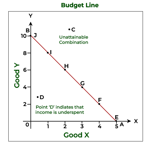
Budget Line, also referred to as the “budget constraint,” is a fundamental concept in consumer theory that represents all possible combinations of two goods a consumer can afford, given their income and the prices of the goods. It serves as a graphical representation of the trade-offs and choices a consumer faces when allocating their limited resources to maximize utility.

Definition of Budget Line

The budget line is a straight line on a graph where:

• The x-axis represents the quantity of one good (Good X).
• The y-axis represents the quantity of another good (Good Y).

The slope and position of this line are determined by the consumer’s income and the prices of the goods. Mathematically, the equation of the budget line is:

M = Px⋅X + Py⋅Y

Where:

• M = Consumer’s income
• Px​ = Price of Good X
• Py​ = Price of Good Y
• $X$ and $Y$ = Quantities of Goods X and Y.

Characteristics of a Budget Line

1. Negative Slope: The line slopes downward, reflecting the trade-off between the two goods. To consume more of one good, the consumer must reduce consumption of the other.
2. Straight Line: The linear nature indicates constant prices of goods.
3. Intercepts:
   • The x-intercept (when Y=0) shows the maximum quantity of Good X that can be purchased if all income is spent on it (M/Px​).
   • The y-intercept (when X=0) shows the maximum quantity of Good Y that can be purchased (M/Py​).

3. Assumptions Underlying the Budget Line

• Fixed Income: The consumer has a specific, limited income.
• Fixed Prices: The prices of goods are constant during the analysis.
• Rational Behavior: The consumer aims to maximize utility within the budget constraint.

Shifts and Rotations of the Budget Line

The budget line can change due to variations in income or the prices of goods:

a. Changes in Income

• An increase in income shifts the budget line outward (away from the origin), as the consumer can afford more of both goods.
• A decrease in income shifts it inward (toward the origin), reducing purchasing power.

b. Changes in Prices

• A decrease in the price of one good causes the budget line to pivot outward along the axis of that good, increasing the quantity affordable.
• An increase in the price of one good causes the budget line to pivot inward, reducing the affordable quantity of that good.

Practical Example

Suppose a consumer has an income of ₹100. They wish to allocate it between two goods: apples (Px = ₹10) and bananas (Py = ₹5).

1. If the consumer spends all income on apples: X = M/Px = 100/10 = 10
   They can purchase 10 apples and no bananas.
2. If the consumer spends all income on bananas: Y = M/Py = 100/5 = 20
   They can purchase 20 bananas and no apples.

The budget line will connect the points (10, 0) and (0, 20) on a graph. Any point on this line represents a combination of apples and bananas that exhausts the ₹100 income.

Consumer Choices Within the Budget Line

• On the Line: All income is fully utilized. Consumers maximize utility by choosing a point on the line based on preferences.
• Inside the Line: Indicates underutilization of income or savings. The consumer is not spending all available resources.
• Outside the Line: Unaffordable combinations, as they exceed the consumer’s income.

Importance of the Budget Line

• Understanding Trade-offs: It helps consumers evaluate the opportunity cost of choosing one good over another.
• Utility Maximization: By combining the budget line with indifference curves, consumers determine the optimal bundle of goods.
• Economic Analysis: Budget lines illustrate consumer behavior, enabling businesses and policymakers to predict demand patterns.

Limitations of the Budget Line

• No Savings or Borrowing: The budget line assumes consumers spend all income without saving or borrowing.
• Static Prices: It doesn’t account for price changes or dynamic market conditions.
• Simplified Preferences: Assumes preferences remain constant during the analysis.