Test of Hypothesis

Hypothesis Testing Concept

Hypothesis testing is a statistical technique that is used in a variety of situations. Though the technical details differ from situation to situation, all hypothesis tests use the same core set of terms and concepts. The following descriptions of common terms and concepts refer to a hypothesis test in which the means of two populations are being compared.

NULL HYPOTHESIS

The null hypothesis is a clear statement about the relationship between two (or more) statistical objects. These objects may be measurements, distributions, or categories. Typically, the null hypothesis, as the name implies, states that there is no relationship.

In the case of two population means, the null hypothesis might state that the means of the two populations are equal.

ALTERNATIVE HYPOTHESIS

Once the null hypothesis has been stated, it is easy to construct the alternative hypothesis. It is essentially the statement that the null hypothesis is false. In our example, the alternative hypothesis would be that the means of the two populations are not equal.

SIGNIFICANCE

The significance level is a measure of the statistical strength of the hypothesis test. It is often characterized as the probability of incorrectly concluding that the null hypothesis is false.

The significance level is something that you should specify up front. In applications, the significance level is typically one of three values: 10%, 5%, or 1%. A 1% significance level represents the strongest test of the three. For this reason, 1% is a higher significance level than 10%.

POWER

Related to significance, the power of a test measures the probability of correctly concluding that the null hypothesis is true. Power is not something that you can choose. It is determined by several factors, including the significance level you select and the size of the difference between the things you are trying to compare.

Unfortunately, significance and power are inversely related. Increasing significance decreases power. This makes it difficult to design experiments that have both very high significance and power.

TEST STATISTIC

The test statistic is a single measure that captures the statistical nature of the relationship between observations you are dealing with. The test statistic depends fundamentally on the number of observations that are being evaluated. It differs from situation to situation.

DISTRIBUTION OF THE TEST STATISTIC

The whole notion of hypothesis rests on the ability to specify (exactly or approximately) the distribution that the test statistic follows. In the case of this example, the difference between the means will be approximately normally distributed (assuming there are a relatively large number of observations).

ONE-TAILED VS. TWO-TAILED TESTS

Depending on the situation, you may want (or need) to employ a one- or two-tailed test. These tails refer to the right and left tails of the distribution of the test statistic. A two-tailed test allows for the possibility that the test statistic is either very large or very small (negative is small). A one-tailed test allows for only one of these possibilities.

In an example where the null hypothesis states that the two population means are equal, you need to allow for the possibility that either one could be larger than the other. The test statistic could be either positive or negative. So, you employ a two-tailed test.

The null hypothesis might have been slightly different, namely that the mean of population 1 is larger than the mean of population 2. In that case, you don’t need to account statistically for the situation where the first mean is smaller than the second. So, you would employ a one-tailed test.

CRITICAL VALUE

The critical value in a hypothesis test is based on two things: the distribution of the test statistic and the significance level. The critical value(s) refer to the point in the test statistic distribution that give the tails of the distribution an area (meaning probability) exactly equal to the significance level that was chosen.

DECISION

Your decision to reject or accept the null hypothesis is based on comparing the test statistic to the critical value. If the test statistic exceeds the critical value, you should reject the null hypothesis. In this case, you would say that the difference between the two population means is significant. Otherwise, you accept the null hypothesis.

P-VALUE

The p-value of a hypothesis test gives you another way to evaluate the null hypothesis. The p-value represents the highest significance level at which your particular test statistic would justify rejecting the null hypothesis. For example, if you have chosen a significance level of 5%, and the p-value turns out to be .03 (or 3%), you would be justified in rejecting the null hypothesis.

Hypothesis testing was introduced by Ronald Fisher, Jerzy Neyman, Karl Pearson and Pearson’s son, Egon Pearson.   Hypothesis testing is a statistical method that is used in making statistical decisions using experimental data.  Hypothesis Testing is basically an assumption that we make about the population parameter.

Hypothesis Testing is done to help determine if the variation between or among groups of data is due to true variation or if it is the result of sample variation. With the help of sample data we form assumptions about the population, then we have to test our assumptions statistically. This is called Hypothesis testing.

Key terms and concepts:

(i) Null hypothesis: Null hypothesis is a statistical hypothesis that assumes that the observation is due to a chance factor.  Null hypothesis is denoted by; H0: μ1 = μ2, which shows that there is no difference between the two population means.

(ii) Alternative hypothesis: Contrary to the null hypothesis, the alternative hypothesis shows that observations are the result of a real effect.

(iii) Level of significance: Refers to the degree of significance in which we accept or reject the null-hypothesis.  100% accuracy is not possible for accepting or rejecting a hypothesis, so we therefore select a level of significance that is usually 5%.

(iv) Type I error: When we reject the null hypothesis, although that hypothesis was true.  Type I error is denoted by alpha.  In hypothesis testing, the normal curve that shows the critical region is called the alpha region.

(v) Type II errors: When we accept the null hypothesis but it is false.  Type II errors are denoted by beta.  In Hypothesis testing, the normal curve that shows the acceptance region is called the beta region.

(vi) Power: Usually known as the probability of correctly accepting the null hypothesis.  1-beta is called power of the analysis.

(vii) One-tailed test: When the given statistical hypothesis is one value like H0: μ1 = μ2, it is called the one-tailed test.

(viii) Two-tailed test: When the given statistics hypothesis assumes a less than or greater than value, it is called the two-tailed test.

Importance of Hypothesis Testing

Hypothesis testing is one of the most important concepts in statistics because it is how you decide if something really happened, or if certain treatments have positive effects, or if groups differ from each other or if one variable predicts another. In short, you want to proof if your data is statistically significant and unlikely to have occurred by chance alone. In essence then, a hypothesis test is a test of significance.

Possible Conclusions

Once the statistics are collected and you test your hypothesis against the likelihood of chance, you draw your final conclusion. If you reject the null hypothesis, you are claiming that your result is statistically significant and that it did not happen by luck or chance. As such, the outcome proves the alternative hypothesis. If you fail to reject the null hypothesis, you must conclude that you did not find an effect or difference in your study. This method is how many pharmaceutical drugs and medical procedures are tested.

Steps in Hypothesis Testing

Step 1: State the Null Hypothesis

The null hypothesis can be thought of as the opposite of the “guess” the research made (in this example the biologist thinks the plant height will be different for the fertilizers).  So the null would be that there will be no difference among the groups of plants.  Specifically in more statistical language the null for an ANOVA is that the means are the same

Step 2: State the Alternative Hypothesis

The reason we state the alternative hypothesis this way is that if the Null is rejected, there are many possibilities.

For example, [Math Processing Error] is one possibility, as is [Math Processing Error]. Many people make the mistake of stating the Alternative Hypothesis as:  [Math Processing Error] which says that every mean differs from every other mean. This is a possibility, but only one of many possibilities. To cover all alternative outcomes, we resort to a verbal statement of ‘not all equal’ and then follow up with mean comparisons to find out where differences among means exist.  In our example, this means that fertilizer 1 may result in plants that are really tall, but fertilizers 2, 3 and the plants with no fertilizers don’t differ from one another.  A simpler way of thinking about this is that at least one mean is different from all others.

Step 3: Set [Math Processing Error]

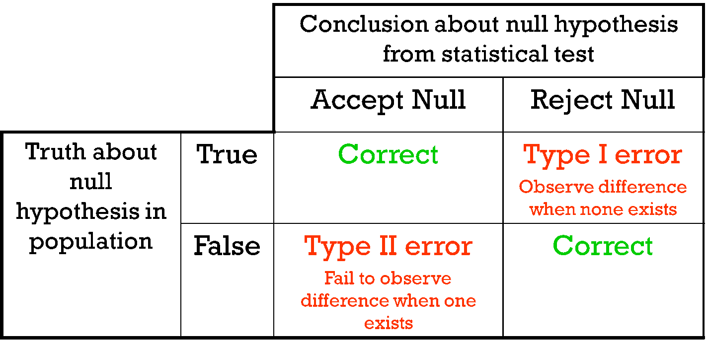
If we look at what can happen in a hypothesis test, we can construct the following contingency table:

	In Reality
Decision	H0 is TRUE	H0 is FALSE
Accept H0	OK	Type II Error β = probability of Type II Error
Reject H0	Type I Error α = probability of Type I Error	OK

You should be familiar with type I and type II errors from your introductory course.  It is important to note that we want to set [Math Processing Error] before the experiment (a-priori) because the Type I error is the more ‘grevious’ error to make. The typical value of [Math Processing Error] is 0.05, establishing a 95% confidence level. For this course we will assume [Math Processing Error] =0.05.

Step 4: Collect Data

Remember the importance of recognizing whether data is collected through an experimental design or observational. 

Step 5: Calculate a test statistic

For categorical treatment level means, we use an F statistic, named after R.A. Fisher. We will explore the mechanics of computing the Fstatistic beginning in Lesson 2. The F value we get from the data is labeled F_calculated.

Step 6: Construct Acceptance / Rejection regions

As with all other test statistics, a threshold (critical) value of F is established. This F value can be obtained from statistical tables, and is referred to as F_critical or [Math Processing Error].  As a reminder, this critical value is the minimum value for the test statistic (in this case the F test) for us to be able to reject the null. 

The F distribution, [Math Processing Error], and the location of Acceptance / Rejection regions are shown in the graph below:

Step 7: Based on steps 5 and 6, draw a conclusion about H₀

If the F_calculated from the data is larger than the Fα, then you are in the Rejection region and you can reject the Null Hypothesis with (1-α) level of confidence.

Note that modern statistical software condenses step 6 and 7 by providing a p-value. The p-value here is the probability of getting an F_calculated even greater than what you observe. If by chance, the F_calculated = [Math Processing Error], then the p-value would exactly equal to α. With larger F_calculated values, we move further into the rejection region and the p-value becomes less than α. So the decision rule is as follows:

If the p-value obtained from the ANOVA is less than α, then Reject H₀ and Accept H_A.