Theory of interest

1. Productivity Theory:

According to productivity theory, interest can be defined as a reward for availing the services of capital for the production purpose.

Labor that is having good amount of capital produces more as compared to the labor who is not assisted by good amount of capital.

For example, farmer having tractor to plough the field produces more as compared to the farmer who does not have it. Thus, interest is the payment for the productivity of capital.

However, the productivity theory is criticized on the following grounds:

  1. Focuses only on the causes for what the interest is paid, not on the determination of interest rates.
  2. Assumes that interest is paid due to the productivity of capital. In such a case, pure interest should vary as per the productivity of the capital. However, pure interest is the same in money market during the same period of time.
  3. Lays emphasis on the demand of interest, but ignores the supply side of capital.
  4. Fails to explain how the interest is paid for the loan borrowed for consumption purposes.

2. Abstinence or Waiting Theory:

The abstinence theory was propounded by Senior. According to him, interest is a reward for abstinence. When an individual saves money out of his/her income and lends it to other individual, he/she makes sacrifice. The term sacrifice implies that the individual refrains from consuming his/her whole income that he/she could spent easily. Senior advocated that abstaining from consumption is unpleasant. Therefore, the lender must be rewarded for this. Thus, as per Senior, interest can be regarded as the reward for refraining from the use of capital.

Abstinence theory was also criticized by a number of economists. According to the theory, an individual feels unpleasant when they save as it reduces his/her consumption. However, rich people do not feel unpleasant while saving because they are able to meet their requirements.

Therefore, Marshall has replaced the term abstinence with waiting and described saving in terms of waiting. He states that saving is done by transferring the present requirement to the future and the person needs to wait for meeting those requirements. However, people do not want to wait rather they are motivated to save money by providing a certain amount of interest.

3. Austrian or Agio Theory:

Austrian theory is also termed as psychological theory of interest. This theory was advocated by John Rae and Bohm Bawerk in an Austrian school. According to Austrian theory, interest came into existence because present goods are preferred over future goods. Therefore, the present goods have premium with them in the form of interest. In other words, present satisfaction is of greater concern as compared to future satisfaction.

Therefore, future satisfaction has certain type of discount if compared with present satisfaction. The interest is the discounted amount that is required to be paid for motivating people to invest or transfer their present requirements to future. For example, an individual has to make a choice between two options.

He/she can either have Rs. 500 now or the same amount after a year. In such a case, he/she would prefer to have Rs. 500 in present. However, in case, the individual has a choice of getting Rs. 500 in present and Rs. 600 after one year.

In such a case, he/she would be more inclined toward getting Rs. 600 after a year. Thus, the extra payment of Rs. 100 would compensate the sacrifice involved in delaying his/her present satisfaction. The extra payment of Rs. 100 in the given case is considered as interest.

Agio theory’ has been criticized by various economists on the following grounds:

  1. Lays too much emphasis on the supply aspect and ignores the demand aspect
  2. Does not focus on the determination of rate of interest

4. Classical or Real Theory:

Classical theory helps in the determination of rate of interest with the help of demand and supply forces. Demand refers to the demand of investment and supply refers to the supply of savings. According to this theory, rate of interest refers to the amount paid for saving.

Therefore, the rate of interest can be determined with the help of demand for saving money to be invested in the capital goods and the supply of savings. Let us understand the concept of demand of investment. Capital goods are used for the production of consumer goods and provide returns continuously for many years.

However, a certain degree of uncertainty is associated with capital goods due to their future use. In addition, operation and maintenance costs are involved in using capital goods. This makes organizations to calculate the net expected return on the marginal cost that is represented as the percentage of cost of capital good.

In case, an organization has similar type of capital goods, then the increase in one more capital good would not yield them high revenue. The increase in the rate of interest would result in the fall of demand of capital goods.

Figure-18 shows the demand for capital investment:

4.1

In Figure-18, MRP represents the marginal revenue productivity curve. When the demand of capital is OM, then the rate of interest is Or. The net rate of return becomes equal to the current rate of interest (Or) at the OM demand of capital.

In case, the rate of interest decreases to Or’, then the demand of capital increases to OM’. The net rate of return is equal to Or’ when the amount of capital demanded is OM’. The demand for capital goods increases with a decrease in the rate of interest.

On the other hand, the supply of capital increases by the amount saved by an individual and the saving is done by transferring the present requirement to the future requirement. The rate of interest would increase with the increase in the amount of saving by an individual.

The rate of interest can be determined with the help of demand of investment and supply of savings. It would be the point of equilibrium where demand and supply intersects each other or get equal.

Figure-19 shows the determination of rate of interest with the help of demand and supply curves:

4.2

In Figure-19, SS is the supply curve of saving and II is the demand curve of investment that intersect each other at Or rate of interest with quantity of saving and investment is OM. OM represents the amount that is lent, borrowed and used for investment. The rate of interest can be changed by changing the demand and supply of savings and investment.

The classical theory is criticized by Keynes due to various reasons, which are as follows:

  1. Assumes the full employment of resources, which is not true in reality. This is because if one resource is reduced from one production process, then it would be utilized for other production process. On the contrary, if resources are available in abundant, then there is no need to save them.
  2. Assumes that investment can be increased only when individuals reduce their consumption. This is because if the consumption is less, then the saving would increase, which would lead to the increase in investment. However, if the demand of capital goods decreases, then the incentive to produce capital goods would also decrease. This would result in the decrease of investment.
  3. Assumes that there is no change in the income level of an individual. Thus, according to classical theory, saving and investment become equal due to change in rate of interest. However, according to Keynes theory, savings and investment become equal because of changes occur in the income level of an individual.

5. Loanable Fund Theory:

Loanable fund theory agrees with the view that time preference plays an important role in determining the occurrence of interest. This theory is also termed as neo-classical theory of interest. According to neo-classical economists, interest is the amount paid for loanable funds. It focuses on the determination of rate of interest with the help of demand and supply of loanable funds in the credit market. Let us understand the concept of supply of loanable funds.

The supply of loanable funds depends on the following factors:

  1. Savings:

Act as one of the sources of loanable funds. The loanable funds in the form of saving are classified as ex-ante saving and Robertsonian sense. Ex-ante saving refers to the saving that an individual plans according to his/her expected income and expenditure in the starting of a year or financial year or for a month.

On the other hand, Robertsonian sense refers to the saving that is produced by taking the difference of previous period income and present period consumption. In both the types of savings, the savings are different at different rate of interest. Savings are dependent on the income level that vanes with the rate of interest. The increase in the rate of interest would result in the increase of the level of saving and vice versa.

In the context of organizations, the amount left after distributing the profit in the form of dividends is termed as the saving of an organization. The savings of an organization depends on the rate of interest prevailing in the market. Increased rate of interest would encourage organizations to increase savings instead of borrowing money from loan market.

2. Dishoarding:

Involves reduction in the money stock of an organization. Therefore, in the previous money stock, the liquidity of money is high that can be utilized in the present time as loanable funds. The higher the rate of interest, the more would be the money dishoarded and vice versa.

3. Credit by bank:

Refers to the loan provided by bank to the organizations. Banks can increase or decrease the money lend to an organization on the basis of certain criteria. The supply of loanable funds increases with the increase in the money created by banks. The supply curve is interest elastic for loanable funds. The higher the rate of interest, the more the bank would lend money and vice versa.

4. Disinvestment:

Refers to the situation when the existing capital goods of an organization are reduced or the stock of the organization is less than the previous stock. In such a condition, the fund that is used for the replacement purposes are used as loanable funds.

According to Bober, ”Disinvestment is encouraged by the somewhat by a high rate of interest on loanable funds. When the rate is high, some of the current capital may not produce a marginal revenue product to match this rate of interest. The firm may decide to let this capital run down and to put the depreciation finds in the ban market”

After determining the factors that influence the supply of loanable funds, let us study the demand for loanable funds. The demand for loanable funds depends on investment, consumption, and hoarding of income. Organizations require loanable funds to a greater extent for expanding the stock of capital goods, such as machines and buildings.

The demand for loanable funds depends on the extent to which organizations require loanable funds. Interest is the price at which the loanable funds can be bought. Organizations require loanable funds at which the net rate of return on capital goods is equal to the rate of interest.

The higher rate of interest demotivates organizations to buy capital goods or expand their stock of capital goods. Therefore, the demand of loanable funds is interest elastic for organizations; therefore, the demand curve would slope downwards.

Another major constituent of demand for loanable funds is the requirement of funds b) individuals for consumption. Generally, individuals require loanable fund when they desire to purchase something out of their budget or the consumer goods that they cannot afford from their present income. The lower the rate of interest, the higher would be the demand for loanable goods. Therefore, the demand for loanable funds is interest elastic for individuals; thus the demand curve slopes downward.

Along with organizations and individuals, there are some people who require loanable goods for hoarding purposes. Hoarding refers to the holding of some part of income by the individuals for future use. In hoarding, the supplier and buyer of loanable funds is the same person.

A person may want to hold funds when the rate of interest is low. On the contrary, he/she may use his/her funds by investing in new projects, when the rate of interest is high. Therefore, the demand of loanable funds is interest elastic for hoarding purpose; thus, the demand curve slopes downward.

Figure-20 shows the interaction between the demand and supply curve of loanable funds to reach at equilibrium position:

4.3

In Figure-20, DH represents dishoarding curve, BM is bank credit curve, S represents saving curve, and DI is disinvestment curve. LS represent the supply of loanable funds, which is produced by summing up the DH, BM, S, and DI curve. Similarly, H represents hoarding, C is consumption, and I is investment, which together form LD.

In Figure-20, LD is the demand for loanable funds. The point at which the demand and supply curve of loanable funds intersect each other is termed as equilibrium point (E). At point E, the rate of interest is OR with ON loanable funds. Therefore, OR would be the equilibrium rate of interest in the credit market.
Law of Diminishing Marginal utility

“Other things remaining the same when a person takes successive units of a commodity, the marginal utility diminishes constantly”.

The marginal utility of a commodity diminishes at the consumer gets larger quantities of it. Marginal utility is the change in the total utility resulting from one unit change in the consumption of a commodity per unit of time.

Assumptions:

Following are the assumptions of the law of diminishing marginal utility.

  1. The utility is measurable and a person can express the utility derived from a commodity in qualitative terms such as 2 units, 4 units and 7 units etc.
  2. A rational consumer aims at the maximization of his utility.
  3. It is necessary that a standard unit of measurement is constant
  4. A commodity is being taken continuously. Any gap between the consumption of a commodity should be suitable.
  5. There should be proper units of a good consumed by the consumer.
  6. It is assumed that various units of commodity homogeneous in characteristics.
  7. The taste of the consumer remains same during the consumption o the successive units of commodity.
  8. Income of the consumer remains constant during the operation of the law of diminishing marginal utility.
  9. It is assumed that the commodity is divisible.
  • There should be not change in fashion. For example, if there is a fashion of lifted shirts, then the consumer may have no utility in open shirts.
  • It is assumed that the prices of the substitutes do not change. For example, the demand for CNG increases due to rise in the prices of petroleum and these price changes effect the utility of CNG.

Explanation with Schedule and Diagram:

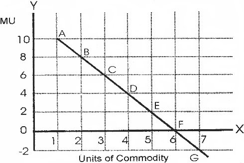
We assume that a man is very thirsty. He takes the glasses of water successively. The marginal utility of the successive glasses of water decreases, ultimately, he reaches the point of satiety. After this point the marginal utility becomes negative, if he is forced further to take a glass of water. The behavior of the consumer is indicated in the following schedule:

Units of commodity

Marginal utility

Total utility

1st glass 10 10
2nd glass 8 18
3rd glass 6 24
4th glass 4 28
5th glass 2 30
6th glass 0 30
7th glass -2 28

On taking the 1st glass of water, the consumer gets 10 units of utility, because he is very thirsty. When he takes 2nd glass of water, his marginal utility goes down to 8 units because his thirst has been partly satisfied. This process continues until the marginal utility drops down to zero which is the saturation point. By taking the seventh glass of water, the marginal utility becomes negative because the thirst of the consumer has already been fully satisfied.

The law of diminishing marginal utility can be explained by the following diagram drawn with the help of above schedule:

In the above figure, the marginal utility of different glasses of water is measured on the y-axis and the units (glasses of water) on X-axis. With the help of the schedule, the points A, B, C, D, E, F and G are derived by the different combinations of units of the commodity (glasses of water) and the marginal utility gained by different units of commodity. By joining these points, we get the marginal utility curve. The marginal utility curve has the downward negative slope. It intersects the X-axis at the point of 6th unit of the commodity. At this point “F” the marginal utility becomes zero. When the MU curve goes beyond this point, the MU becomes negative. So there is an inverse functional relationship between the units of a commodity and the marginal utility of that commodity.

Limitations:

The limitations or exceptions of the law of diminishing marginal utility are as follows:

  1. The law does not hold well in the rare collections. For example, collection of ancient coins, stamps etc.
  2. The law is not fully applicable to money. The marginal utility of money declines with richness but never falls to zero.
  3. It does not apply to the knowledge, art and innovations.
  4. The law is not applicable for precious goods.
  5. Historical things are also included in exceptions to the law.
  6. Law does not operate if consumer behaves in irrational manner. For example, drunkard is said to enjoy each successive peg more than the previous one.
  7. Man is fond of beauty and decoration. He gets more satisfaction by getting the above merits of the commodities.
  8. If a dress comes in fashion, its utility goes up. On the other hand its utility goes down if it goes out of fashion.
  9. The utility increases due to demonstration. It is a natural element.

Importance of the Law of Diminishing Marginal Utility:

The importance or the role of the law of diminishing marginal utility is as follows:

  1. By purchasing more of a commodity the marginal utility decreases. Due to this behaviour, the consumer cuts his expenditures to that commodity.
  2. In the field of public finance, this law has a practical application, imposing a heavier burden on the rich people.
  3. This law is the base of some other economic laws such as law of demand, elasticity of demand, consumer surplus and the law of substitution etc.
  4. The value of commodity falls by increasing the supply of a commodity. It forms a basis of the theory of value. In this way prices are determined

Equi Marginal Utility

The Law of equi-marginal Utility is another fundamental principle of Econo­mics. This law is also known as the Law of substitution or the Law of Maxi­mum Satisfaction. We know that human wants are unlimited whereas the means to satisfy these wants are strictly limited. It, therefore’ becomes necessary to pick up the most urgent wants that can be satisfied with the money that a consumer has. Of the things that he decides to buy he must buy just the right quantity. Every prudent consumer will try to make the best use of the money at his disposal and derive the maximum satisfaction.

Explanation of the Law

In order to get maximum satisfaction out of the funds we have, we carefully weigh the satisfaction obtained from each rupee ‘had we spend If we find that a rupee spent in one direction has greater utility than in another, we shall go on spending money on the former commodity, till the satisfaction derived from the last rupee spent in the two cases is equal.

It other words, we substitute some units of the commodity of greater utility tor some units of the commodity of less utility. The result of this substitution will be that the marginal utility of the former will fall and that of the latter will rise, till the two marginal utilities are equalized. That is why the law is also called the Law of Substitution or the Law of equimarginal Utility.

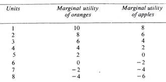
Suppose apples and oranges are the two commodities to be purchased. Suppose further that we have got seven rupees to spend. Let us spend three rupees on oranges and four rupees on apples. What is the result? The utility of the 3rd unit of oranges is 6 and that of the 4th unit of apples is 2. As the marginal utility of oranges is higher, we should buy more of oranges and less of apples. Let us substitute one orange for one apple so that we buy four oranges and three apples.

Now the marginal utility of both oranges and apples is the same, i.e., 4. This arrangement yields maximum satisfaction. The total utility of 4 oranges would be 10 + 8 + 6 + 4 = 28 and of three apples 8 + 6 + 4= 18 which gives us a total utility of 46. The satisfaction given by 4 oranges and 3 apples at one rupee each is greater than could be obtained by any other combination of apples and oranges. In no other case does this utility amount to 46. We may take some other combinations and see.

We thus come to the conclusion that we obtain maximum satisfaction when we equalize marginal utilities by substituting some units of the more useful for the less useful commodity. We can illustrate this principle with the help of a diagram.

Diagrammatic Representation:

In the two figures given below, OX and OY are the two axes. On X-axis OX are represented the units of money and on the Y-axis marginal utilities. Suppose a person has 7 rupees to spend on apples and oranges whose diminishing marginal utilities are shown by the two curves AP and OR respectively.

The consumer will gain maximum satisfaction if he spends OM money (3 rupees) on apples and OM’ money (4 rupees) on oranges because in this situation the marginal utilities of the two are equal (PM = P’M’). Any other combination will give less total satisfaction.

Let the purchase spend MN money (one rupee) more on apples and the same amount of money, N’M'( = MN) less on oranges. The diagram shows a loss of utility represented by the shaded area LN’M’P’ and a gain of PMNE utility. As MN = N’M’ and PM=P’M’, it is proved that the area LN’M’P’ (loss of utility from reduced consumption of oranges) is bigger than PMNE (gain of utility from increased consumption of apples). Hence the total utility of this new combination is less.

We then, conclude that no other combination of apples and oranges gives as great a satisfaction to the consumer as when PM = P’M’, i.e., where the marginal utilities of apples and oranges purchased are equal, with given amour, of money at our disposal.

Limitations of the Law of Equimarginal Utility

Like other economic laws, the law of equimarginal utility too has certain limitations or exceptions. The following are the main exception.

(i) Ignorance

If the consumer is ignorant or blindly follows custom or fashion, he will make a wrong use of money. On account of his ignorance he may not know where the utility is greater and where less. Thus, ignorance may prevent him from making a rational use of money. Hence, his satisfaction may not be the maximum, because the marginal utilities from his expenditure can­not be equalised due to ignorance.

(ii) Inefficient Organisation

In the same manner, an incompetent organ­iser of business will fail to achieve the best results from the units of land, labour and capital that he employs. This is so because he may not be able to divert expenditure to more profitable channels from the less profitable ones.

(iii) Unlimited Resources

The law has obviously no place where this resources are unlimited, as for example, is the case with the free gifts of nature. In such cases, there is no need of diverting expenditure from one direction to another.

(iv) Hold of Custom and Fashion

A consumer may be in the strong clutches of custom, or is inclined to be a slave of fashion. In that case, he will not be able to derive maximum satisfaction out of his expenditure, because he cannot give up the consumption of such commodities. This is specially true of the conventional necessaries like dress or when a man is addicted to some into­xicant.

(v) Frequent Changes in Prices

Frequent changes in prices of different goods render the observance of the law very difficult. The consumer may not be able to make the necessary adjustments in his expenditure in a constantly changing price situation.

Consumer’s Surplus

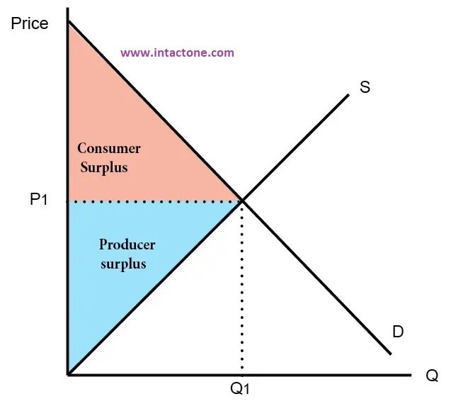
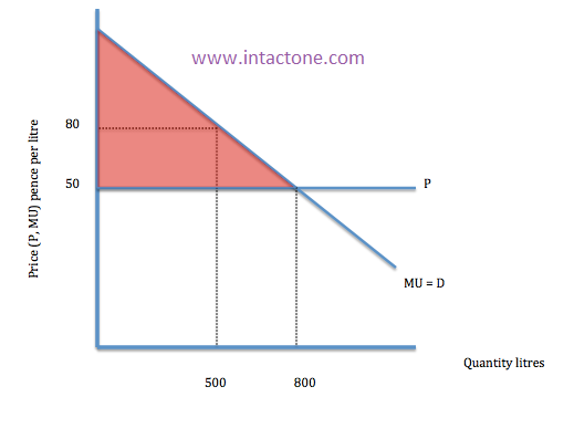
Consumer Surplus is the difference between the price that consumers pay and the price that they are willing to pay. On a supply and demand curve, it is the area between the equilibrium price and the demand curve

For example, if you would pay 76p for a cup of tea, but can buy it for 50p; your consumer surplus is 26p

Diagram of Consumer Surplus

Producer Surplus

  • This is the difference between the price a firm receives and the price it would be willing to sell it at.
  • Therefore it is the difference between the supply curve and the market price.

Consumer Surplus and Marginal Utility

The demand curve is derived from our marginal utility. If the marginal utility of a good is greater than the price, then that is our consumer surplus.

  1. Firms can reduce consumer surplus if they have market power. This enables them to raise prices above the competitive equilibrium.
  2. In a monopoly, a firm will maximise profits by reducing consumer surplus.
  3. Another way to reduce consumer surplus is to engage in price discrimination. Charging different prices to different groups of consumers. Those with inelastic demand will see their consumer surplus reduced. More on Price discrimination. To completely eliminate consumer surplus, a firm would need to engage in first-degree price discrimination this means charging the consumer the highest price they are willing to pay.
  4. To gain market power, a firm could advertise to create brand loyalty, this will make demand more inelastic

Significance of consumer surplus

  • In competitive markets, firms have to keep prices relatively low, enabling consumers to gain consumer surplus. If markets were not competitive, the consumer surplus would be less and there would be greater inequality.
  • A lower consumer surplus leads to higher producer surplus and greater inequality.
  • Consumer surplus enables consumers to purchase a wider choice of goods.

Decision Support Systems, Attributes, Characteristics, Classification, Types, Advantages, Disadvanatages

Decision Support system (DSS) is a computerized program used to support determinations, judgments, and courses of action in an organization or a business. A DSS sifts through and analyzes massive amounts of data, compiling comprehensive information that can be used to solve problems and in decision-making.

Typical information used by a DSS includes target or projected revenue, sales figures or past ones from different time periods, and other inventory- or operations-related data.

A DSS can be used by operations management and planning levels in an organization to compile information and data and synthesize it into actionable intelligence. This allows the end user to make more informed decisions at a quicker pace.

The DSS is an information application that produces comprehensive information. This is different from an operations application, which would be used to collect the data in the first place. A DSS is primarily used by mid- to upper-level management, and it is key for understanding large amounts of data.

For example, a DSS could be used to project a company’s revenue over the upcoming six months based on new assumptions about product sales. Due to the large amount of variables that surround the projected revenue figures, this is not a straightforward calculation that can be done by hand. A DSS can integrate multiple variables and generate an outcome and alternate outcomes, all based on the company’s past product sales data and current variables.

The primary purpose of using a DSS is to present information to the customer in a way that is easy to understand. A DSS system is beneficial because it can be programed to generate many types of reports, all based on user specifications. A DSS can generate information and output it graphically, such as a bar chart that represents projected revenue, or as a written report.

As technology continues to advance, data analysis is no longer limited to large bulky mainframes. Since a DSS is essentially an application, it can be loaded on most computer systems, including laptops. Certain DSS applications are also available through mobile devices. The flexibility of the DSS is extremely beneficial for customers who travel frequently. This gives them the opportunity to be well-informed at all times, which in turn provides them with the ability to make the best decisions for their company and customers at any time.

Process of Decision Support Systems (DSS):

  1. Data Input:

Gathering relevant data from various sources, both internal and external.

  1. Data Processing:

Analyzing and processing data using models, algorithms, and analytical tools.

  1. Knowledge Base:

Utilizing a knowledge base to store relevant information, rules, and decision criteria.

  1. User Interface:

Providing a user-friendly interface for querying and interacting with the system.

  1. Model Execution:

Executing models and simulations to generate insights and scenarios.

  1. Results Presentation:

Presenting results through reports, dashboards, and visualizations.

  1. User Feedback:

Gathering feedback from users to improve system performance.

Attributes of a DSS

  • Adaptability and flexibility
  • High level of Interactivity
  • Ease of use
  • Efficiency and effectiveness
  • Complete control by decision-makers
  • Ease of development
  • Extendibility
  • Support for modeling and analysis
  • Support for data access
  • Standalone, integrated, and Web-based

Characteristics of a DSS

  • Support for decision-makers in semi-structured and unstructured problems.
  • Support for managers at various managerial levels, ranging from top executive to line managers.
  • Support for individuals and groups. Less structured problems often requires the involvement of several individuals from different departments and organization level.
  • Support for interdependent or sequential decisions.
  • Support for intelligence, design, choice, and implementation.
  • Support for variety of decision processes and styles.
  • DSSs are adaptive over time.

Benefits of DSS

  • Improves efficiency and speed of decision-making activities.
  • Increases the control, competitiveness and capability of futuristic decision-making of the organization.
  • Facilitates interpersonal communication.
  • Encourages learning or training.
  • Since it is mostly used in non-programmed decisions, it reveals new approaches and sets up new evidences for an unusual decision.
  • Helps automate managerial processes.

Disadvantages of Decision Support Systems:

  • Complex Implementation:

Implementing DSS may require specialized skills and technical expertise.

  • High Initial Costs:

The initial investment in DSS development and implementation can be substantial.

  • Dependency on Data Quality:

DSS effectiveness heavily relies on the quality and accuracy of input data.

  • Resistance to Change:

Users may resist adopting new decision-making processes facilitated by DSS.

  • Security Concerns:

DSS may handle sensitive information, raising security and privacy issues.

  • Overemphasis on Technology:

Overreliance on technology may overlook the human element in decision-making.

  • Limited Flexibility:

Some DSS may lack flexibility to adapt to rapidly changing business environments.

  • Integration Challenges:

Integrating DSS with existing systems may pose compatibility and integration challenges.

  • Learning Curve:

Users may face a learning curve when adopting new DSS tools and interfaces.

  • Maintenance Requirements:

Regular maintenance and updates are necessary to keep DSS effective and up-to-date.

Components of a DSS

(i) Database Management System (DBMS)

To solve a problem the necessary data may come from internal or external database. In an organization, internal data are generated by a system such as TPS and MIS. External data come from a variety of sources such as newspapers, online data services, databases (financial, marketing, human resources).

(ii) Model Management System

It stores and accesses models that managers use to make decisions. Such models are used for designing manufacturing facility, analyzing the financial health of an organization, forecasting demand of a product or service, etc.

(iii) Support Tools

Support tools like online help; pulls down menus, user interfaces, graphical analysis, error correction mechanism, facilitates the user interactions with the system.

Classification of DSS

There are several ways to classify DSS. Hoi Apple and Whinstone classifies DSS as follows:

(i) Text Oriented DSS

It contains textually represented information that could have a bearing on decision. It allows documents to be electronically created, revised and viewed as needed.

(ii) Database Oriented DSS

Database plays a major role here; it contains organized and highly structured data.

(iii) Spreadsheet Oriented DSS

It contains information in spread sheets that allows create, view, modify procedural knowledge and also instructs the system to execute self-contained instructions. The most popular tool is Excel and Lotus 1-2-3.

(iv) Solver Oriented DSS

It is based on a solver, which is an algorithm or procedure written for performing certain calculations and particular program type.

(v) Rules Oriented DSS

It follows certain procedures adopted as rules.

(vi) Rules Oriented DSS

Procedures are adopted in rules oriented DSS. Export system is the example.

(vii) Compound DSS

It is built by using two or more of the five structures explained above.

Types of DSS

(i) Status Inquiry System

It helps in taking operational, management level, or middle level management decisions, for example daily schedules of jobs to machines or machines to operators.

(ii) Data Analysis System

It needs comparative analysis and makes use of formula or an algorithm, for example cash flow analysis, inventory analysis etc.

(iii) Information Analysis System

In this system data is analyzed and the information report is generated. For example, sales analysis, accounts receivable systems, market analysis etc.

(iv) Accounting System

It keeps track of accounting and finance related information, for example, final account, accounts receivables, accounts payables, etc. that keep track of the major aspects of the business.

(v) Model Based System

Simulation models or optimization models used for decision-making are used infrequently and creates general guidelines for operation or management.

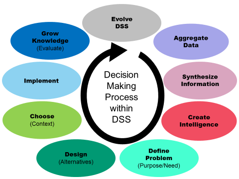
Decision Support Systems Role in Decision making process

  1. Data Aggregation and Analysis:

    • Role of DSS:
      • Gathers and aggregates relevant data from various sources.
      • Analyzes data using advanced modeling and analytical techniques.
    • Impact on Decision Making:
      • Provides decision-makers with a comprehensive view of relevant information.
      • Enables in-depth analysis for better-informed decisions.
  2. Scenario Simulation:

    • Role of DSS:
      • Allows for the creation and simulation of different decision scenarios.
      • Models the potential outcomes of various decision options.
    • Impact on Decision Making:
      • Assists decision-makers in understanding the consequences of different choices.
      • Supports proactive decision-making by exploring potential scenarios.
  1. Decision Modeling and Optimization:

    • Role of DSS:
      • Utilizes mathematical models to represent decision problems.
      • Optimizes decision variables to achieve the best outcomes.
    • Impact on Decision Making:
      • Provides decision-makers with quantifiable and objective insights.
      • Optimizes resource allocation and decision parameters.
  1. Access to Real-Time Information:

    • Role of DSS:
      • Integrates with systems to provide real-time data updates.
      • Ensures decision-makers have access to the latest information.
    • Impact on Decision Making:
      • Enables timely decision-making based on current and relevant data.
      • Supports agility and responsiveness in dynamic business environments.
  1. User-Friendly Interfaces:

    • Role of DSS:
      • Provides intuitive and user-friendly interfaces for interaction.
      • Allows users to easily input queries and interact with the system.
    • Impact on Decision Making:
      • Reduces the learning curve for users, fostering widespread adoption.
      • Enhances accessibility for decision-makers across different levels.
  1. Collaboration Support:

    • Role of DSS:
      • Facilitates collaboration by allowing multiple users to interact with the system.
      • Supports shared decision-making processes.
    • Impact on Decision Making:
      • Encourages teamwork and collective decision-making.
      • Improves communication and coordination among decision-makers.
  1. Information Presentation:

    • Role of DSS:
      • Presents insights through visualizations, reports, and dashboards.
      • Transforms complex data into easily understandable formats.
    • Impact on Decision Making:
      • Enhances comprehension by presenting information in a digestible manner.
      • Supports quick and effective decision-making.
  1. Risk Assessment and Mitigation:

    • Role of DSS:
      • Assesses potential risks associated with decision options.
      • Recommends strategies to mitigate identified risks.
    • Impact on Decision Making:
      • Helps decision-makers make informed choices while considering potential risks.
      • Supports the development of risk-conscious decision-making strategies.
  1. Feedback Mechanism:

    • Role of DSS:
      • Establishes a feedback loop for continuous improvement.
      • Collects feedback from users to enhance system performance.
    • Impact on Decision Making:
      • Enables continuous learning and improvement in decision-making processes.
      • Incorporates user insights for refining decision support functionalities.

Executive Information Systems, Process, Disadvantages, Role in Decision making process

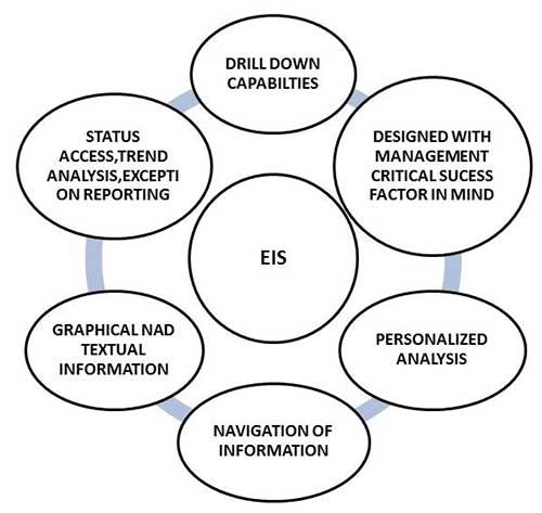
An Executive Information System can be defined as a specialized Decision Support System. This type of the system generally includes the various hardware, software, data, procedures and the people. With the help of all this, the top level executives get a great support in taking and performing the various types of the decisions. The executive information system plays a very important role in obtaining the data from the different sources, then help in the integration and the aggregation of this data. After performing these steps the resulting information is displayed in such a pattern that is very easy to understand.

Executive information system is ‘a computer based system that serves the information that is needed by the various top executives. It provides very rapid access to the timely information and also offers the direct access to the different management reports.’

Executive Information System is very user friendly in the nature. It is supported at a large extent by the graphics.

Executive support system can be defined as the comprehensive executive support system that goes beyond the Executive Information System and also includes communications, office automation, analysis support etc.

According to Watson, Executive Information System / executive support system depends on some of the factors that can be summarized as the follows

  1. Internal factors
  • Need for the timely information.
  • Need for the improved communications.
  • Need for the access to the operational data.
  • Need for the rapid status updates on the various business activities.
  • Need for the access to the corporate database.
  • Need for very accurate information.
  • Need for the ability to identify the various historical trends.
  1. External Factors
  • Increasing and intensifying the global competition.
  • Rapidly changing the business environment.
  • Need to be more proactive.
  • Need to access the external database.
  • Increasing the various government regulations.

Characteristics of the Executive Information System

  1. Informational characteristics
  • Flexibility and ease of use
  • Provides the timely information with the short response time and also with the quick retrieval
  • Produces the correct information
  • Produces the relevant information
  • Produces the validated information
  1. User interface/orientation characteristics
  • Consists of the sophisticated self help
  • Contains the user friendly interfaces consisting of the graphic user
  • Can be used from many places
  • Offers secure reliable, confidential access along with the access procedure
  • Is very much customized
  • Suites the management style of the individual executives
  1. Managerial / executive characteristics
  • Supports the over all vision, mission and the strategy
  • Provides the support for the strategic management
  • Sometimes helps to deal with the situations that have a high degree of risk
  • Is linked to the value added business processes
  • Supports the need/ access for/ to the external data/ databases
  • Is very much result oriented in the nature

Capabilities of Executive Information System

(i) Helps in accessing the aggregated or macro or global information.

(ii) Provides the user with an option to use the external data extensively.

(iii) Enables analysis of the address and the hoc queries.

(iv) Shows the trends, the ratios and the various deviations.

(v) Helps in incorporating the graphic and the text in the same display, which helps to have a better view.

(vi) It helps in the assessment of the historical as also the latest data.

(vii) Problem indicators can be highlighted with the help of the Executive Information System / executive support system.

(viii) Open ended problem explanation with the written interpretations can be done with the help of the Executive Information System / executive support system.

(ix) Offers management by the exception reports.

(x) Utilizes the hyper text and the hyper media.

(xi) Offers generalized computing.

(xii) Offers telecommunications capacity.

Executive Information System Process

  • Data Collection:

EIS gathers data from various internal and external sources, including databases, reports, and external data feeds.

  • Data Processing:

The collected data undergoes processing, including validation, aggregation, and transformation to ensure accuracy and relevance.

  • Data Storage:

Processed data is stored in a centralized repository, often a data warehouse, for easy retrieval and analysis.

  • Information Retrieval:

Executives can query the EIS to retrieve specific information based on their needs. The system uses user-friendly interfaces for ease of interaction.

  • Data Analysis and Reporting:

EIS provides tools for data analysis, generating reports, summaries, and visualizations that offer insights into key performance indicators (KPIs) and relevant metrics.

  • Trend Identification:

The system identifies trends and patterns within the data, allowing executives to understand historical performance and anticipate future developments.

  • Decision Support:

EIS assists executives in decision-making by providing relevant and timely information. It may include decision support tools and models for scenario analysis.

  • Alerts and Notifications:

EIS monitors predefined thresholds and conditions, triggering alerts or notifications to executives when significant events or deviations occur.

  • Strategic Planning Support:

EIS contributes to strategic planning by offering insights into market trends, competitive intelligence, and the organization’s overall performance.

  • Integration with External Data:

EIS often integrates with external data sources, such as industry reports, economic indicators, and market research, to provide a comprehensive view.

  • Customization for Executives:

EIS is customizable to meet the specific needs and preferences of individual executives, allowing them to focus on the information most relevant to their roles.

  • User Interface and Accessibility:

EIS features user-friendly interfaces that provide easy access to information, ensuring that executives can quickly navigate and retrieve the data they require.

  • Feedback Mechanism:

Executives can provide feedback on the usefulness and relevance of the information provided, contributing to system refinement and improvement.

  • Security Measures:

EIS incorporates robust security measures to safeguard sensitive executive-level information and ensure data confidentiality.

Benefits of Executive Information System

(i) Achievement of the various organizational objectives.

(ii) Facilitates access to the information by integrating many sources of the data.

(iii) Facilitates broad, aggregated perspective and the context.

(iv) Offers broad highly aggregated information.

(v) User’s productivity is also improved to a large extent.

(vi) Communication capability and the quality are increased.

(vii) Provides with the better strategic planning and the control.

(viii) Facilitates pro-active rather than a reactive response.

(ix) Provides the competitive advantage.

(x) Encourages the development of a more open and active information culture.

(xi) The cause of a particular problem can be founded.

Executive Information System Disadvantages

  • Costly Implementation:

The initial investment in designing, implementing, and maintaining an EIS can be substantial, including costs for hardware, software, training, and ongoing support.

  • Complexity and Customization:

EIS can be complex to implement, and customization to fit specific executive needs may require a high level of expertise and effort.

  • Dependency on Data Quality:

The effectiveness of EIS is highly dependent on the quality of the underlying data. Inaccurate or incomplete data can lead to flawed insights and decisions.

  • Integration Challenges:

Integrating EIS with existing information systems within the organization can be challenging, especially in environments with diverse data sources and formats.

  • Resistance to Change:

Executives and organizational members may resist adapting to new technologies and processes, potentially hindering the successful adoption of EIS.

  • Security Concerns:

EIS often deals with sensitive and confidential information. Ensuring robust security measures is crucial to prevent unauthorized access and protect against data breaches.

  • Learning Curve:

Executives and users may face a learning curve when using new EIS tools and interfaces, which can temporarily impact productivity.

  • Overemphasis on Technology:

Overreliance on EIS may lead to a reduction in the importance of human intuition and experience in decision-making, potentially overlooking nuanced aspects.

  • Limited Flexibility:

Some EIS solutions may lack flexibility to adapt quickly to changes in business environments or evolving executive information needs.

  • Maintenance Requirements:

Ongoing maintenance is essential for EIS to remain effective. This includes updates, troubleshooting, and ensuring compatibility with evolving technologies.

  • Data Overload:

EIS, when presenting a large volume of information, may lead to information overload for executives, making it challenging to focus on critical data points.

  • Potential for Misinterpretation:

Executives may misinterpret presented information, especially if they lack a comprehensive understanding of the data sources, models, or assumptions used.

  • Dependency on IT Support:

Executives may become overly dependent on IT support for system-related issues, potentially slowing down decision-making in case of technical problems.

  • Ethical Considerations:

The use of EIS raises ethical concerns related to the privacy and responsible use of sensitive information, requiring organizations to establish clear guidelines and policies.

Executive Information System Role in Decision making process

  • Access to Critical Information:

EIS provides top executives with quick and easy access to critical information relevant to their roles. This information includes key performance indicators (KPIs), financial metrics, market trends, and strategic data.

  • Real-Time Data Monitoring:

Executives can monitor real-time data through EIS, allowing them to stay informed about the current state of the organization and external factors that may impact decision-making.

  • Strategic Planning Support:

EIS assists in strategic planning by offering insights into long-term trends, market dynamics, and competitive intelligence. Executives can align organizational goals with available resources and external opportunities.

  • Decision Support Tools:

EIS incorporates decision support tools such as data analytics, modeling, and scenario analysis. These tools help executives evaluate various decision options and their potential outcomes.

  • Performance Measurement:

Executives can use EIS to measure the performance of different departments, business units, or projects, enabling data-driven assessments and informed decision-making.

  • Risk Management:

EIS supports risk management by identifying potential risks and uncertainties. Executives can use this information to develop strategies for mitigating risks and making more informed decisions.

  • Facilitation of Communication:

EIS facilitates communication among top executives by providing a centralized platform for sharing information, insights, and collaborative decision-making.

  • Aggregation of Information:

EIS aggregates information from diverse sources, including internal databases, external market reports, and operational systems. This aggregation provides a comprehensive view for decision-makers.

  • Customization for Executives:

EIS allows executives to customize dashboards and reports based on their specific information needs. This ensures that executives focus on the most relevant data for their decision-making processes.

  • Performance Evaluation:

Executives can use EIS to evaluate the performance of strategic initiatives, allowing for adjustments and refinements in alignment with organizational goals.

  • Alerts and Notifications:

EIS includes alert mechanisms that notify executives of critical events or deviations from established benchmarks, enabling proactive decision-making.

  • Benchmarking:

Executives can compare the organization’s performance against industry benchmarks and competitors, aiding in strategic positioning and goal setting.

  • Data Visualization:

EIS employs data visualization techniques such as charts and graphs to present complex information in a visually comprehensible format, aiding executives in understanding trends and patterns.

  • Feedback Loop:

EIS establishes a feedback loop where executives can provide feedback on the effectiveness of decisions made and the relevance of information presented, contributing to continuous improvement.

Meaning of Correlation, Importance

Correlation, in the finance and investment industries, is a statistic that measures the degree to which two securities move in relation to each other. Correlations are used in advanced portfolio management, computed as the correlation coefficient, which has a value that must fall between -1.0 and +1.0

A perfect positive correlation means that the correlation coefficient is exactly 1. This implies that as one security moves, either up or down, the other security moves in lockstep, in the same direction. A perfect negative correlation means that two assets move in opposite directions, while a zero correlation implies no relationship at all.

For example, large-cap mutual funds generally have a high positive correlation to the Standard and Poor’s (S&P) 500 Index – very close to 1. Small-cap stocks have a positive correlation to that same index, but it is not as high – generally around 0.8.

However, put option prices and their underlying stock prices will tend to have a negative correlation. As the stock price increases, the put option prices go down. This is a direct and high-magnitude negative correlation.

  • Correlation is a statistic that measures the degree to which two variables move in relation to each other.
  • In finance, the correlation can measure the movement of a stock with that of a benchmark index, such as the Beta.
  • Correlation measures association, but does not tell you if x causes y or vice versa, or if the association is caused by some third (perhaps unseen) factor.

Importance of correlation Analysis

Correlation is very important in the field of Psychology and Education as a measure of relationship between test scores and other measures of performance. With the help of correlation, it is possible to have a correct idea of the working capacity of a person. With the help of it, it is also possible to have a knowledge of the various qualities of an individual.

After finding the correlation between the two qualities or different qualities of an individual, it is also possible to provide his vocational guidance. In order to provide educational guidance to a student in selection of his subjects of study, correlation is also helpful and necessary.

Correlation Statistics and Investing

The correlation between two variables is particularly helpful when investing in the financial markets. For example, a correlation can be helpful in determining how well a mutual fund performs relative to its benchmark index, or another fund or asset class. By adding a low or negatively correlated mutual fund to an existing portfolio, the investor gains diversification benefits.

In other words, investors can use negatively-correlated assets or securities to hedge their portfolio and reduce market risk due to volatility or wild price fluctuations. Many investors hedge the price risk of a portfolio, which effectively reduces any capital gains or losses because they want the dividend income or yield from the stock or security.

Correlation statistics also allows investors to determine when the correlation between two variables changes. For example, bank stocks typically have a highly-positive correlation to interest rates since loan rates are often calculated based on market interest rates. If the stock price of a bank is falling while interest rates are rising, investors can glean that something’s askew. If the stock prices of similar banks in the sector are also rising, investors can conclude that the declining bank stock is not due to interest rates. Instead, the poorly-performing bank is likely dealing with an internal, fundamental issue.

Degrees of Price Discrimination

Price discrimination means charging different prices from different customers or for different units of the same product. In the words of Joan Robinson: “The act of selling the same article, produced under single control at different prices to different buyers is known as price discrimination.” Price discrimination is possible when the monopolist sells in different markets in such a way that it is not possible to transfer any unit of the commodity from the cheap market to the dearer market.

Degrees of price discrimination

Prof. Pigou in his Economics of Welfare describes three degrees of discriminating power which a monopolist may wield. The type of discrimination discussed above is called discrimination of the third degree. We explain below discrimination of the first degree and the second degree.

Discrimination of the First Degree (1st) or Perfect Discrimination

Discrimination of the first degree occurs when a monopolist charges “a different price against all the different units of commodity in. such wise that the price exacted for each was equal to the demand price for it and no consumer’s surplus was left to the buyers.”

Joan Robinson calls it perfect discrimi­nation when the monopolist sells each unit of the product at a separate price. Such discrimination is possible only when consumers are sold the units for which they are prepared to pay the highest price and thus they are not left with any consumer’s surplus.

For perfect price discrimination, two conditions are required

(1) To keep the buyers separate from each other, and

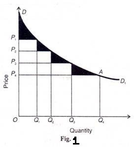
(2) To deal with each buyer on a take-it-or-leave-it basis. When the discriminator of first degree is able to deal with his customers on the above basis, he can transfer the whole of consumers’ surplus to himself. Consider Figure 1. Where DD1 is the demand curve faced by the monopolist. Each buyer is assumed as a price-taker. Suppose the discriminating monopolist sells four units of his product at four different prices:

OQ1 unit at OP1price, Q1Q2 unit at OPprice, Q2Q3 unit at OP3 price and Q3Q4 unit at OP4 price. The total revenue (or price) obtained by him would be OQ4 AD. This area is the maximum expenditure that the consumers are willing to incur to buy all four units of the product under the first-degree discriminator’s all-or-nothing offer. But with no price discrimination under simple monopoly, the monopolist would sell all four units at the uniform price OP4 and thus obtain the total revenue of OQ4AP4.

This area represents the total expenditure that consumers would actually pay for the four units. Thus the difference between what Quantity the consumers were willing to pay (OQ4 AD) under Fig. 1 the take-it-or-leave-it offer of the first degree discrimi­nator and what they actually pay (OQ4AP4) to the simple monopolist, is consumers’ surplus. This is equal to the area of the triangle DAP4.

Thus under the first-degree price discrimination, the entire consumers’ surplus is pocketed by the monopolist when he charges a separate price for each unit of the product. Price discrimination of the first degree is rare and is to be found in such rare products as diamonds, jewels, precious stones, etc. But a monopolist must have full knowledge of the demand curve faced by him and he should know the maximum price that the consumers are willing to pay for each unit of the product he wants to sell.

Discrimination of the Second Degree (2nd) or Multi-part Pricing

In discrimination of the second degree, the monopolist divides the consumers in different slabs or groups or blocks and charges different prices for different slabs of the same product. Since the earlier units of the product have more utility for the consumers than the later ones, the monopolist charges a higher price for the former units and reduces the price for the later units in the respective slabs.

Such discrimination is only possible if the demand of each consumer below a certain maximum price is perfectly inelastic. Electric supply companies in developed countries practice discrimination of the second degree when they charge a high rate for the first slab of kilowatts of electricity consumed. As more electricity is used, the rate falls with subsequent slabs.

Figure 2 illustrates the second degree discrimination, where DD1is the demand curve for electric­ity on the part of domestic consumers in a town. CP3 represents the cost of generating electricity, so that the electricity company charges M1P1 rate per kw. up to OM1 units. For consuming the next M1 to М2 units, the rate is lowered to M2P2. The lowest rate charged is M3P3 for M2 to M3 units. M3P3 is, however, the lowest rate which will be charged even if a con­sumer consumes more than M3 units of electricity.

If the electricity company were to charge only one rate throughout, say M3P3the total revenue would not be maximized. It would be OCP3 M3But by charg­ing different rates for different unit slabs, it gets the total revenue equal to OM3 x P1M1 + OM2 x P2M2 + OM3x P3M3 Thus the second degree discriminator would take away a part of consumers’ surplus covered by the rectangles ABEP1and BCFP2 .The shaded area in three triangles DAP1 Р1ЕР2, and P2FP3 still remains with consumers as their surplus.

The second degree price discrimination is practised by telephone companies, railways, companies supplying water, electricity and gas in developed countries where these services are available in plenty. But it is not found in developing countries like India where such services are scarce.

The differences between the first and second degree price discrimination may be noted. In the first degree discrimination, the monopolist charges a different price for each different unit of the prod­uct. But in second degree discrimination, a number of units in one slab (or group or block) are sold at the lowest price and as the slabs increase, the prices charged by the monopolist are lowered. In the case of the former the monopolist takes away the whole of consumers’ surplus. But in the latter case, the monopolist takes away only a portion of the consumers’ surplus and the other portion is left with the buyer.

Conditions under which Price Discrimination is Possible

Price discrimination is possible under following conditions:

  1. Nature of Commodity

In the first place it is said that price discrimination is possible when the nature of the commodity or service is such that there is no possibility of transference from one market to the other.

That is, the goods sold in the cheaper market cannot be resold in the dearer market; otherwise the monopolist’s purpose will be defeated.

  1. Distance of Two Markets

Price discrimination is possible when the two markets or markets are separated by large distance or tariff barriers, so that it is not possible to transfer goods from a cheaper market to dearer markets. For instance, a monopolist may sell the same product at a higher price in Bombay and lower price in Meerut.

  1. Ignorance of the Consumers

Price discrimination is possible when the consumers are ignorant about price discrimination, they are not aware that in one part of the market prices are lower than in the other part. Thus, he purchases in dearer market, than in cheaper market since he is ignorant of the prices that are prevailing in different markets.

  1. Government Regulation

Price discrimination occurs when the government rules and regulations permit. For instance, according to rules, electricity rates are fixed at higher level for industrial purposes and lower for domestic uses. Similarly, railways charge by law higher fares from first class passengers than from the second class passengers. Hence, price discrimination is possible because of legal sanction.

  1. Geographical Discrimination

Price discrimination may be possible on account of geographical situations. The monopolist may discriminate between home and foreign buyers by selling at lower price in the foreign market than in the domestic market. Geographical discrimination is possible because no unit of the commodity sold in one market can be transferred to another.

  1. Difference in Elasticity of Demand

A commodity may have different elasticity of demand in different markets. Thus, the market of a commodity can be separated on the basis of its elasticity of demand.

Hence, a monopolist can charge different prices in different markets classified on the basis of elasticity of demand, low price is charged where demand is more elastic and high price in the market with the less elastic demand or inelastic demand.

  1. Artificial Difference between Goods

A monopolist may create artificial differences by presenting the same commodity under different names and labels, one for the rich and snobbish buyers and the other for the ordinary customers. For instance, a biscuit manufacturer may wrap small quantity of the biscuits, give it separate name and charge a higher price. Thus, he may charge different price for substantially the same product. He may charge Rs. 2/- for 100 gram wrapped biscuits and Rs. 1.50 for unwrapped biscuits.

error: Content is protected !!